An Introduction to the Kalman Filter - Computer Science

1 An Introduction to the Kalman Filter Greg Welch 1 and Gary Bishop 2 TR 95-041 Department of Computer ScienceUniversity of North Carolina at Chapel HillChapel Hill, NC 27599-3175 Updated: Monday, July 24, 2006 Abstract In 1960, Kalman published his famous paper describing a recursive solution to the discrete-data linear filtering problem. Since that time, due in large part to ad-vances in digital computing, the Kalman Filter has been the subject of extensive re-search and application, particularly in the area of autonomous or assisted Kalman Filter is a set of mathematical equations that provides an efficient com-putational (recursive) means to estimate the state of a process, in a way that mini-mizes the mean of the squared error. The Filter is very powerful in several aspects: it supports estimations of past, present, and even future states, and it can do so even when the precise nature of the modeled system is purpose of this paper is to provide a practical Introduction to the discrete Kal-man Filter .

2 This Introduction includes a description and some discussion of the basic discrete Kalman Filter , a derivation, description and some discussion of the extend-ed Kalman Filter , and a relatively simple (tangible) example with real numbers & results. 1. ~welch 2. ~gb Welch & Bishop, An Introduction to the Kalman Filter2 UNC-Chapel Hill, TR 95-041, July 24, 2006 1 The Discrete Kalman Filter In 1960, Kalman published his famous paper describing a recursive solution to the discrete-data linear filtering problem [Kalman60]. Since that time, due in large part to advances in digital computing, the Kalman Filter has been the subject of extensive research and application, particularly in the area of autonomous or assisted navigation. A very friendly Introduction to the general idea of the Kalman Filter can be found in Chapter 1 of [Maybeck79], while a more complete introductory discussion can be found in [Sorenson70], which also contains some interesting historical narrative.

3 More extensive references include [Gelb74; Grewal93; Maybeck79; Lewis86; Brown92; Jacobs93]. The Process to be Estimated The Kalman Filter addresses the general problem of trying to estimate the state of a discrete-time controlled process that is governed by the linear stochastic difference equation,( )with a measurement that is.( )The random variables and represent the process and measurement noise (respectively). They are assumed to be independent (of each other), white, and with normal probability distributions,( ).( )In practice, the process noise covariance and measurement noise covariance matrices might change with each time step or measurement, however here we assume they are matrix in the difference equation ( ) relates the state at the previous time step to the state at the current step , in the absence of either a driving function or process noise.

4 Note that in practice might change with each time step, but here we assume it is constant. The matrix B relates the optional control input to the state x . The matrix in the measurement equation ( ) relates the state to the measurement z k . In practice might change with each time step or measurement, but here we assume it is constant. The Computational Origins of the Filter We define (note the super minus ) to be our a priori state estimate at step k given knowledge of the process prior to step k , and to be our a posteriori state estimate at step k given measurement . We can then define a priori and a posteriori estimate errors asx n xkA xk1 Buk1 wk1 ++=z m zkH xkvk+=wkvkp w( )N0Q,( ) p v( )N0R,( ) QRnn Ak1 kAnl u l mn HHx k- n x k n zkek-xkx k-, and ekxkx k. Welch & Bishop, An Introduction to the Kalman Filter3 UNC-Chapel Hill, TR 95-041, July 24, 2006 The a priori estimate error covariance is then,( )and the a posteriori estimate error covariance is.

5 ( )In deriving the equations for the Kalman Filter , we begin with the goal of finding an equation that computes an a posteriori state estimate as a linear combination of an a priori estimate and a weighted difference between an actual measurement and a measurement prediction as shown below in ( ). Some justification for ( ) is given in The Probabilistic Origins of the Filter found below.( )The difference in ( ) is called the measurement innovation , or the residual . The residual reflects the discrepancy between the predicted measurement and the actual measurement . A residual of zero means that the two are in complete agreement. The matrix K in ( ) is chosen to be the gain or blending factor that minimizes the a posteriori error covariance ( ). This minimization can be accomplished by first substituting ( ) into the above definition for , substituting that into ( ), performing the indicated expectations, taking the derivative of the trace of the result with respect to K , setting that result equal to zero, and then solving for K.

6 For more details see [Maybeck79; Brown92; Jacobs93]. One form of the resulting K that minimizes ( ) is given by 1 .( )Looking at ( ) we see that as the measurement error covariance approaches zero, the gain K weights the residual more heavily. Specifically,.On the other hand, as the a priori estimate error covariance approaches zero, the gain K weights the residual less heavily. Specifically,. 1. All of the Kalman Filter equations can be algebraically manipulated into to several forms. Equation ( )represents the Kalman gain in one popular []=PkEekekT[ ]=x kx k-zkH x k-x kx k-KzkH x k- ()+=zkH x k- ()H x k-zknm ekKkPk-HTH Pk-HTR+()1 =Pk-HTH Pk-HTR+-----------------------------=RKk Rk0 limH1 =Pk-KkPk-0 lim0=Welch & Bishop, An Introduction to the Kalman Filter4 UNC-Chapel Hill, TR 95-041, July 24, 2006 Another way of thinking about the weighting by K is that as the measurement error covariance approaches zero, the actual measurement is trusted more and more, while the predicted measurement is trusted less and less.

7 On the other hand, as the a priori estimate error covariance approaches zero the actual measurement is trusted less and less, while the predicted measurement is trusted more and Probabilistic Origins of the FilterThe justification for ( ) is rooted in the probability of the a priori estimate conditioned on all prior measurements (Bayes rule). For now let it suffice to point out that the Kalman Filter maintains the first two moments of the state distribution,The a posteriori state estimate ( ) reflects the mean (the first moment) of the state distribution it is normally distributed if the conditions of ( ) and ( ) are met. The a posteriori estimate error covariance ( ) reflects the variance of the state distribution (the second non-central moment). In other words,.For more details on the probabilistic origins of the Kalman Filter , see [Maybeck79; Brown92; Jacobs93].

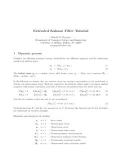
8 The Discrete Kalman Filter AlgorithmWe will begin this section with a broad overview, covering the high-level operation of one form of the discrete Kalman Filter (see the previous footnote). After presenting this high-level view, we will narrow the focus to the specific equations and their use in this version of the Kalman Filter estimates a process by using a form of feedback control: the Filter estimates the process state at some time and then obtains feedback in the form of (noisy) measurements. As such, the equations for the Kalman Filter fall into two groups: time update equations and measurement update equations. The time update equations are responsible for projecting forward (in time) the current state and error covariance estimates to obtain the a priori estimates for the next time step. The measurement update equations are responsible for the feedback for incorporating a new measurement into the a priori estimate to obtain an improved a posteriori time update equations can also be thought of as predictor equations, while the measurement update equations can be thought of as corrector equations.

9 Indeed the final estimation algorithm resembles that of a predictor-corrector algorithm for solving numerical problems as shown below in Figure x k-Pk-zkH x k-x k-zkExk[ ]x k=Exkx k ()xkx k ()T[] xkzk()NExk[ ]Exkx k ()xkx k ()T[],() Nx kPk,().=Welch & Bishop, An Introduction to the Kalman Filter5 UNC-Chapel Hill, TR 95-041, July 24, 2006 Figure 1-1. The ongoing discrete Kalman Filter cycle. The time update projects the current state estimate ahead in time. The measurement update adjusts the projected estimate by an actual measurement at that specific equations for the time and measurement updates are presented below in Table 1-1 and Table notice how the time update equations in Table 1-1 project the state and covariance estimates forward from time step to step . and B are from ( ), while is from ( ). Initial conditions for the Filter are discussed in the earlier first task during the measurement update is to compute the Kalman gain.

10 Notice that the equation given here as ( ) is the same as ( ). The next step is to actually measure the process to obtain , and then to generate an a posteriori state estimate by incorporating the measurement as in ( ). Again ( ) is simply ( ) repeated here for completeness. The final step is to obtain an a posteriori error covariance estimate via ( ).After each time and measurement update pair, the process is repeated with the previous a posteriori estimates used to project or predict the new a priori estimates. This recursive nature is one of the very appealing features of the Kalman Filter it makes practical implementations much more feasible than (for example) an implementation of a Wiener Filter [Brown92] which is designed to operate on all of the data directly for each estimate. The Kalman Filter instead recursively conditions the current estimate on all of the past measurements.