Transcription of ANSYS FLUENT Airfoil Analysis and Tutorial
1 ANSYS FLUENT . Airfoil Analysis and Tutorial ENGR083: Fluid Mechanics II. Terry Yu 5/11/2017. Abstract The NACA 0012 Airfoil was one of the earliest airfoils created. Its mathematically simple shape and age have meant that it is one of the first choices for validating CFD programs, as there is a wealth of data on this particular Airfoil . Though the NACA 0012 Airfoil is not in general use currently due to its relatively poor lift to drag ratio, it remains a useful research tool. It still sees some use, however, in control surfaces and helicopter blades, as it is symmetric and thus has a simple correlation between angle of attack and lift. This project validated methods for using ANSYS FLUENT and created a Tutorial for future E83 students to also analyze this Airfoil .
2 The resulting coefficient of lift plot is remarkably similar to one produced by NASA's Langley Center, while the coefficient of drag plot seems to be in error. This is likely due to our simple viscosity model. Introduction ANSYS FLUENT is part of the ANSYS suite of engineering Analysis software, which includes Mechanical APDL, BladeGen, and many other software packages capable of thermal Analysis , electromagnetic Analysis , and more. FLUENT is also widely recognized as one of the industry standard CFD software packages. Although Solidworks is capable of performing rudimentary CFD Analysis , it is only a rudimentary approach as Solidworks is fundamentally CAD software and is not built with simulation in mind, as ANSYS is. The versatility and capability of ANSYS FLUENT makes it an easy first choice for fluid dynamics Analysis .
3 This project seeks to find a basic understanding of ANSYS FLUENT and develop a Tutorial for future students to also learn from this software. In a previous project, I analyzed the NACA. 0012 Airfoil structurally to understand its deflection due to aerodynamic forces in a helicopter. Thus, I had the model readily available. However, the model was in 3D form, and I had to analyze only a cross section of the Airfoil . Unfortunately, FLUENT 's academic license does not allow for enough meshes to cover the entire 3D Airfoil . This was fortuitous, though, as we were able to corroborate our results with a NASA Langley Center study on the characteristics of the Airfoil . After completing our Analysis , we created a Tutorial to introduce new E83 students to FLUENT .
4 This Tutorial will walk the user through importing the Airfoil model and setting up the boundary conditions for meshing and solving the fluids problem. Due to time, we were unable to implement a Tutorial for modeling or for more simple shapes in FLUENT , which may have been more helpful to novice students. Problem The fundamental problem we are attempting to solve is the modeling of a 2D Airfoil cross section. Given the below figure, how can we determine the lift and drag acting on the Airfoil ? The picture above shows a box with an Airfoil cutout. In order to analyze an Airfoil , my implementation does not implement a wind tunnel and an object suspended in it, although that is a valid approach. Instead, this procedure cuts out an Airfoil shape from a bounding box, and meshes the box.
5 The entire box is then divided into finite elements, and the fluid dynamics equations are solved. By examining the fluid properties near the Airfoil cutout, the lift and drag can be determined. We have wind tunnel tests and other software validations from the Langley center, so we are able to compare our lift and drag results to validated results, and see if there were any mistakes in our protocol or software implementation. For our Airfoil , we are working in the turbulent regime, with Re = 6million. Our speed is M= , which converts to about 51 m/s. This region is essentially incompressible, but the NASA website cautions against running incompressible flow, as the results may differ. From determined lift and drag forces, we can calculate the lift and drag coefficients.
6 These are plotted against the angle of attack, and compared to available data. A close match confirms that our implementation and procedure are correct. Theory First, we must determine the regime that our Analysis is in. Our reference data is for Re = 6. million, which is far into the turbulent region.. =.. where =density, =velocity, =dynamic viscosity, and L is the characteristic length, which for our Airfoil is the chord. With known viscosity, density, and speed, we can calculate the length. The values we used were: kg = m3. m = 51. s kg = x 10 5. m s = m To determine the coefficients of drag and lift, we use the following equations from the NASA. website1. where L and D are the lift and drag, is the free stream density, is the free stream velocity, and A is the reference area (in 2-D it is reference length, or area per unit span).
7 It should be noted that these differ from the equations derived in class. Our solver has the energy equation enabled, which enables compressible flow. To model compressible flow, we use the ideal gas law to determine the density at any given point. 1. FLUENT models turbulence with the Reynolds average Navier-Stokes Equations (RANS). This is one of the most common approaches to computing flows. Other methods exist to model flow, such as Detached Eddy Simulation or Large Eddy simulation. However, while more accurate, RANS is far less computationally intensive and yields close enough results for the scales that we are working at. Below is the full Reynolds averaged momentum equation. At each iteration, this equation is solved for all the mesh quadrilaterals.
8 The Reynolds stress tensor describes unknowns introduced by modeling and must be related to average flow quantities. To calculate the Reynolds stress tensor, we must use eddy viscosity models. The Boussinesq hypothesis states that Reynold stresses can be modeled with an eddy viscosity . This is reasonable for simple turbulent shear flows such as boundary layers, round jets, mixing layers, channel flows, but for complex flows we need to fully solve the Reynolds Stress tensor, which is computationally intense. The eddy viscosity above must be resolved to complete the RANS equations. Below are our choices of models. There are many methods of calculating eddy viscosity, and we have chosen the Spalart-Allmaras equation for its simplicity.
9 RANS based models Eddy viscosity models Spalart-Allmaras is the computationally simplest model. It is economical for large meshes, but performs poorly for 3D flows, free shear flows, and flows with strong separation. It is suitable for mildly complex (quasi-2D) external/internal flows and boundary layer flows under pressure gradient ( airfoils, wings, airplane fuselages, missiles, ship hulls), which is perfect for our simulations. The other equations are more suitable to complex flows, such as turbomachinery, flows with high separation, flows with high strain rates, or flows with high swirl rates. The Spalart-Allmaras equations are adequate for our purposes, but any more complex Analysis than simple shapes in a uniform flow. The Spalart-Allmaras equations can be characterized as where eddy viscosity is obtained from By solving this equation, FLUENT can solve for the eddy viscosity.
10 With the eddy viscosity, the Reynolds stress tensor is known, and once the stress tensor is known, the entire Reynolds- Averaged Navier Stokes equations can be solved. Results At the proscribed Re = 6 million, we obtained the following graph for the lift coefficient: This was overlaid with the NASA coefficient of lift chart. Our values are in orange. This shows very good agreement, with only some discontinuities in the stall region. The coefficient of drag vs coefficient of lift graph was also plotted: This was also overlaid with the NASA coefficient of lift chart. Our values are in green. This shows fairly poor agreement with the NASA values. Although we managed the same general shape, we are off by a fair amount. Following are sample contours and streamlines from a 10 degree angle case.