Transcription of Applications of the Gauss-Newton Method
1 Applications of the Gauss-Newton MethodAs will be shown in the following section, there are a plethora of Applications for an iterative process for solving a non-linear least-squares approximation problem. It can be used as a Method of locating a single point or, as it is most often used, as a way of determining how well a theoretical model fits a set of experimental data points. By solving the system of non-linear equations we obtain the best estimates of the unknown variables in a theoretical model. We are then able to plot this function along with the data points and see how well these data points fit the theoretical first problem to be solved involved the finding of a single point. Say, for example, that there are a set of m beacons located at positions (pk,qk).
2 Each of these beacons is at a given distance dk from their origin. Given these positions and distances, we expect that the distance to the origin of each point is given by the following equation:D(u,v)= ((u pk)2+(v qk)2)Where u and v are the x and y coordinates of the origin. As mentioned before, we are not attempting to find the exact location of the origin, by the very nature of a least-squares problem this solution does not exist or else we wouldn't need to bother with the program at all, we are merely looking for the values u and v that minimize the sum of the squares of the residuals that is, the values that minimize the function:S= k=1mrk2 Where r, in this particular scenario, is given by the equation:rk=dk ((u pk)2+(v qk)2)To test to see if the Gauss-Newton Method will actually find the proper solution to this problem, we begin with a system to which we know the solution, in practice this would not be done but as a way to test the success of the Method and the code this is appropriate.
3 A vector z of 100 random points in the range zero to two pi was generated in MATLAB; our values for p and q were then given by p=cos(z) and q=sin(z). This generated a circular set of points whose distances to the origin, known to be located at (0,0), was 1. Because the Gauss-Newton Method requires the calculation of the Jacobian matrix of r, we first analytically determined the partial derivates of r with respect to both u and v:( r)( u)=(u pk) ((u pk)2+(v qk)2)( r)( v)=(v qk) ((u pk)2+(v qk)2)In the program shown below, the Jacobian is calculated at each iteration using the newest approximations of p and q in the function df at the bottom of the code. Once the partial derivates of the Jacboian were determined, the Gauss-Newton Method could be applied.
4 Since we know that the actual origin is at (0,0) the initial guesses for u and v were chosen to be: u= and v= (in the program the values for u and v are stored in the column vector a). function [unknowns,steps,S] = GaussNewton()%GaussNewton- uses the Gauss-Newton Method to perform a non-linear least%squares approximation for the origin of a circle of points% Takes as input a row vector of x and y values, and a column vector of% initial guesses. partial derivatives for the jacobian must entered below% in the df functionformat longtol = 1e-8; %set a value for the accuracymaxstep = 30; %set maximum number of steps to run forz = 2*pi*rand(100,1); %create 100 random pointsp = cos(z); %create a circle with those pointsq = sin(z); d = ones(100,1); %set distance to origin as 1 for all pointsa = [ ; ]; %set initial guess for originm=length(p); %determine number of functionsn=length(a); %determine number of unkownsaold = a;for k=1:maxstep %iterate through process S = 0.
5 For i=1:m for j=1:n J(i,j) = df(p(i),q(i),a(1,1),a(2,1),j); %calculate Jacobian JT(j,i) = J(i,j); %and its trnaspose end end Jz = -JT*J; %multiply Jacobian and %negative transpose for i=1:m r(i,1) = d(i) - sqrt((a(1,1)-p(i))^2+(a(2,1)-q(i))^2);%c alculate r S = S + r(i,1)^2; %calculate sum of squares of residuals end S g = Jz\JT; %mulitply Jz inverse by J transpose a = aold-g*r; %calculate new approximation unknowns = a; err(k) = a(1,1)-aold(1,1); %calculate error if (abs(err(k)) <= tol); %if less than tolerance break break end aold = a; %set aold to aendsteps = k;hold allplot(p,q,'r*') %plot the data pointsplot(a(1,1),a(2,1),'b*') %plot the approximation of the origin(expect it to be 0,0)title(' Gauss-Newton Approximation of Origin of Circular Data Points') %set axis lables, title and legendxlabel('X')ylabel('Y')legend('Data Points',' Gauss-Newton Approximation of Origin')hold offerrratio(3:k) = err(2:k-1).
6 /err(3:k); %determine rate of convergenceend function value = df(p,q,a1,a2,index) %calculate partialsswitch index case 1 value = (2*a1 - 2*p)* *((a1-p)^2+(a2-q)^2)^( ); case 2 value = (2*a2 - 2*q)* *((a1-p)^2+(a2-q)^2)^( );endendThe program generates two things. First, a plot of the beacons (pk,qk) and the final approximation of the origin at point (u,v) and second, the values of u and v stored in the column vector unknowns as well as the number of steps the program ran before reaching the desired precision (steps) and the sum of the squares of the residuals at each iteration (stored in S).The final values of u and v were returned as: u= * and v= * , while the total number of steps run was 3. It should be noted that although both the exact values of u and v and the location of the points on the circle will not be the same each time the program is run, due to the fact that random points are generated, the program will still return values that are extremely close to the origin.
7 By examining the plot shown and the final values of u and v it is clear to see that the Gauss-Newton Method and its implementation in the above code are successful in solving the non-linear system of equations. Furthermore, because we are trying to minimize the sum of the squares of the residuals, we can look at these values at each iteration of the program to determine if we are getting a more accurate value for our unknowns. Shown below is a table with the number of steps and the value for S at each of these steps:Iteration table shows that the Gauss-Newton Method has drastically decreased the value S that we are attempting to minimize to a degree of precision that is near machine precision. It should be noted that not all values of S will reach this degree of accuracy.
8 Because we are dealing with an example where the value of the unknowns exists, we can obtain a value for S that is extremely close to zero. Usually, as mentioned before, the problems dealt with will not have an obtainable solution, merely an approximation of the closes value to the that success of both the Method and the implementation have been validated, it is possible to expand the previous example to an origin that is impossible to determine exactly. To do this, an almost identical version of the previous mentioned code was implemented. However, this time instead of generating points in a circle about a known origin, 100 entirely random points were generated within the range zero to one, with 100 randomly generated distances. In this case, it is impossible to determine the exact location to the origin; however, the Gauss-Newton may provide us with a way to approximate the best possible solution.
9 The code to do this is shown below along with the plot generated and the final values returned for u and [unknowns,steps,S] = GaussNewtonSquare()%GaussNewton- uses the Gauss-Newton Method to perform a non-linear least%squares approximation for the origin of a circle of points% Takes as input a row vector of x and y values, and a column vector of% initial guesses. partial derivatives for the jacobian must entered below% in the df functionformat longtol = 1e-8; %set a value for the accuracymaxstep = 50; %set maximum number of steps to run forp = rand(100,1); %generate random values for p and q between zero and 1 q = rand(100,1); d = rand(100,1); %generate random distances to origina = [ ; ]; %set initial guess for originm=length(p); %determine number of functionsn=length(a); %determine number of unkownsaold = a;for k=1:maxstep %iterate through process S = 0; for i=1:m for j=1:n J(i,j) = df(p(i),q(i),a(1,1),a(2,1),j).
10 %calculate Jacobian JT(j,i) = J(i,j); %and its trnaspose end end Jz = -JT*J; %multiply Jacobian and %negative transpose for i=1:m r(i,1) = d(i) - sqrt((a(1,1)-p(i))^2+(a(2,1)-q(i))^2);%c alculate r S = S + r(i,1)^2; %calculate sum of squares of residuals end S g = Jz\JT; %mulitply Jz inverse by J transpose a = aold-g*r; %calculate new approximation unknowns = a; err(k) = a(1,1)-aold(1,1); %calculate error if (abs(err(k)) <= tol); %if less than tolerance break break end aold = a; %set aold to aendsteps = k;hold allplot(p,q,'r*') %plot the data pointsplot(a(1,1),a(2,1),'b*') %plot the approximation of the origin(expect it to be 0,0)title(' Gauss-Newton Approximation of Randomly Placed Beacons') %set axis lables, title and legendxlabel('X')ylabel('Y')legend('Beac ons',' Gauss-Newton Approximation of Origin')hold offerrratio(3:k) = err(2:k-1).