Transcription of Applying Deep Neural Networks to Financial Time Series ...
1 Applying Deep Neural Networks to FinancialTime Series ForecastingAllison KoeneckeAbstractFor any Financial organization, forecasting economic and Financial vari-ables is a critical operation. As the granularity at which forecasts are needed in-creases, traditional statistical time Series models may not scale well; on the otherhand, it is easy to incorrectly overfit machine learning models. In this chapter, wewill describe the basics of traditional time Series analyses, discuss how Neural net-works work, show how to implement time Series forecasting using Neural Networks ,and finally present an example with real data from Microsoft. In particular, Mi-crosoft successfully approached revenue forecasting using deep Neural networksconjointly with curriculum learning, which achieved a higher level of precision thanis possible with traditional Introduction to Time Series AnalysisTime seriesare simply Series of data points ordered by time.
2 We first discuss themost commonly-used traditional (non- Neural network) models, and then commenton pitfalls to avoid when formulating these Common Methods for Stationary Time SeriesTime Series analyses can be classified as parametric or non-parametric, where theformer assumes a certain underlying stationary stochastic process, whereas the lat-ter does not and implicitly estimates covariance of the process. We mostly focus onInstitute for Computational & Mathematical Engineering, Stanford, California, USA, Koeneckeparametric modeling within this chapter. Note that there are trade-offs in dealingwith parametric modeling. Specifically, significant data cleaning is often necessaryto transform non-stationary time Series into stationary data that can be used withparametric models; tuning parameters is also often a difficult and costly other machine learning methods exist, such as running a basic linear regres-sion or random forest using time Series features ( , lags of the given data, timesof day, etc.)
3 Stationary time serieshave constant mean and variance (that is, statistical prop-erties do not change over time). The Dickey-Fuller test [1] is used to test for sta-tionarity; specifically, it tests the null hypothesis of a unit root being present in anautoregressive modelsare regressions on the time Series itself, lagged by a certainnumber of timesteps. An AR(1) model, with a time lag of one, is defined asyt= yt 1+ut, forytbeing the time Series with time indext, being the coefficient,andutbeing the error =1 in the autoregressive model above, then a unit root is present, in whichcase the data are non-stationary. Suppose we find that this is the case; how can wethen convert the time Series to be stationary in order to use a parametric model?There are several tricks to doing high autocorrelation is found, one can instead perform analyses on the firstdifference of the data, which isyt yt 1. If it appears that the autocorrelation is sea-sonal ( , there are periodic fluctuations over days, months, quarters, years, etc.)
4 ,one can perform de-seasonalization. This is often done with the STL method (Sea-sonal and Trend Decomposition using Loess) [2], which decomposes a time seriesinto its seasonal, trend, and residual parts; these three parts can either additivelyor multiplicatively form the original time Series . The STL method is especially ro-bust because the seasonal component can change over time, and outliers will notaffect the seasonal or trend components (as they will mostly affect the residual com-ponent). Once the time Series is decomposed into the three parts, one can removethe seasonality component, run the model, and post hoc re-incorporate seasonal-ity. While we focus on STL throughout this chapter, it is worth mentioning thatother common decomposition methods in economics and finance include TRAMO-SEATS [3], X11 [4], and Hodrick-Prescott [5].Recall that stationarity also requires constant variance over time; the lack thereofis referred to as heteroskedasticity.
5 To resolve this issue, a common suggestion is toinstead studylog(yt), which has lower Common ModelsMoving averagecalculation simply takes an average of values from timeti kthroughti, for each time indexi>k. This is done to smooth the original time seriesand make trends more apparent. A largerkresults in a smoother Deep Neural Networks to Financial Time Series Forecasting3 Exponential smoothingnon-parametrically assigns exponentially decreasing weightsfor historical observations. In this way, new data have higher weights for forecast-ing. Exponential smoothing (ETS) is explicitly defined asst= xt+(1 )st 1,t>0(1)where the smoothing algorithm output isst, which is initialized tos0=x0, andxtis the original time Series sequence. The smoothing parameter 0 1 allows oneto set how quickly weights decrease over historical observations. In fact, we can per-form exponential smoothing recursively; if twice, then we introduce an additionalparameter as the trend smoothing factor in double exponential smoothing.
6 Ifthrice (as in triple exponential smoothing ), we introduce a third parameter asthe seasonal smoothing factor for a specified season length. One downside, though,is that historical data are forgotten by the model relatively the Autoregressive Integrated Moving Average [6], one of the mostcommon parametric models. We have already defined autoregression and movingaverage, which respectively take parametersAR(p)wherepis the maximum lag,andMA(q)whereqis the error lag. If we combine just these two concepts, weget ARMA, where are parameters of the autoregression, are parameters of themoving average, and are error terms assumed to be independent and identicallydistributed (from a normal distribution centered at zero). ARMA is as follows:Yt 1Yt 1 .. pYt p= t+ 1 t 1+..+ q t q(2)ARMA can equivalently be written as follows, with lag operatorL:(1 p i=1 iLi)Yt= (1+q i=1 iLi) t(3)From this, we can proceed to ARIMA, which includes integration.
7 Specifically,it regards the order of integration: that is, the number of differences to be taken fora Series to be rendered stationary. IntegrationI(d)takes parameterd, the unit rootmultiplicity. Hence, ARIMA is formulated as follows:(1 p d i=1 iLi)(1 L)dYt= (1+q i=1 iLi) t(4) Forecasting Evaluation MetricsWe often perform the above modeling so that we can forecast time Series into thefuture. But, how do we compare whether a model is better or worse at forecasting?We first designate a set of training data, and then evaluate predictions on a separatelyheld-out set of test data. Then, we compare our predictions to the test data andcalculate an evaluation KoeneckeHold-out setsIt is important to perform cross-validation properly such that themodel only sees training data up to a certain point in time, and does not get to cheat by looking into the future; this mistake is referred to as data leakage.
8 Because we may only have a single time Series to work with, and our predictionsare temporal, we cannot simply arbitrarily split some share of the data into a trainingset, and another share into validation and test sets. Instead, we use a walk-forwardsplit [7] wherein validation sets are a certain number of timesteps forward in timefrom the training sets. If we train a model on the time Series from timet0toti,then we make predictions for timesti+1throughti+k(wherek=1 in Figure 1, andprediction onti+4only is shown in Figure 2) for some chosenk. We calculate anerror on the predictions, and then enlarge the training set and iteratively calculateanother error, and so on, continuously walking forward in time until the end ofthe available data. In general, this idea is called the rolling window process, andallows us to do multiple-fold validation. The question that remains now is how tocalculate prediction 1 Cross validation with 1-step-ahead fore-casts; training data are in blue, and test dataare in red.
9 Specifically, forecasts are only madeone timestep further than the end of the trainingdata [8]Fig. 2 Cross validation with 4-step-ahead fore-casts. Forecasting can be done for any specifictimestep ahead, or range of timesteps, so longas the training and test split are preserved assuch [8]Evaluation metricsWe can use several different evaluation metrics to calculateerror on each of the validation folds formed as described above. Letyibe the actualtest value, and yibe the prediction for theithfold overnfolds. The below commonmetrics can be aggregated across folds to yield one final metric:1. Mean Absolute Error: ni=1|yi yi|n2. Mean Absolute Percentage Error:1n ni=1 yi yiyi 3. Mean Squared Error:1n ni=1(yi yi)24. R squared: 1 ni=1(yi yi)2 ni=1(yi 1n ni=1yi)2 Applying Deep Neural Networks to Financial Time Series Common PitfallsWhile there are many ways for time Series analyses to go wrong, there are four com-mon pitfalls that should be considered: using parametric models on non-stationarydata, data leakage, overfitting, and lack of data overall.
10 These pitfalls extend to thedata cleaning steps that will be used with Neural Networks , which are described inSection 2. Below we recap what can be done to ameliorate these dataEnsure that data is transformed prior to modeling. We sug-gest several methods in Section , such as order differences, seasonality removal,and logarithmic transformations. Further to this, trends can also be removed ( , bysubtracting the overall mean of a time Series ), smoothing can be done by replacingthe time Series with a moving average, and other transformations may be useful aswell ( , standardization or Box-Cox). In general, it is also good practice to cleandata by removing leakageConfirm that cross-validation is done correctly, so that the modeldoes not see any future data relative to the timestep it is predicting. In particular, ifde-meaning the data to make it stationary, ensure that means are calculated only overeach training data batch, rather than across the entire duration of the time training data points may predict overly well, so the model mayoverfit to those rather than generalizing, resulting in lower accuracy in the test regression-based analyses, regularizers (such as Lasso and Ridge) or featureselection can help.