Transcription of Approximations to the Stochastic Burgers Equation
1 Approximations to the Stochastic Burgers EquationMartin Hairer, Jochen Voss24th May 2010 AbstractThis article is devoted to the numerical study of various finite difference approximationsto the Stochastic Burgers Equation . Of particular interest in the one-dimensional case isthe situation where the driving noise is white both in space and in time. We demonstratethat in this case, different finite difference schemes converge to different limiting processesas the mesh size tends to zero. A theoretical explanation of this phenomenon is given andwe formulate a number of conjectures for more general classes of equations , supported bynumerical : Stochastic Burgers Equation , correction term, numerical approximationSubject classification:60H35, 60H15, 35K551 IntroductionThis article studies several finite difference schemes for the viscous Stochastic Burgers Equation : tu(x,t) = 2xu g(u) xu+ (x,t), x [0,2 ], t 0.
2 (1)In this Equation , denotes space-time white noise, that is the centred, distribution-valued Gaus-sian random variable such thatE( (x,t) (y,s))= (t s) (x y). We will always endow thisequation with periodic boundary conditions and we will consider solutionsutaking values eitherinRor inRn(in which casegis matrix-valued in general).Motivations for studying the Stochastic Burgers Equation are manifold. Just to name a few,it is used to model vortex lines in high-temperature superconductors [BFG+94], dislocations indisordered solids and kinetic roughening of interfaces in epitaxial growth [Bar96], formation oflarge-scale structures in the universe [GSS85, SZ89], constructive quantum field theory [BCJL94],etc. Since in the case = 0 andg(u) uthis Equation is furthermore explicitly solvable viathe Hopf-Cole transform (u= xv/v, wherevsolves the heat Equation ), it comes as no surprisethat a wealth of numerical and analytical results are available.
3 From a purely mathematicalpoint of view, let us mention for example the well-posedness results from [BCF91, BCJL94,DPDT94, Gy o98, Kim06] and the ergodicity results obtained in [TZ06, GM05]. One remarkableachievement was the construction of a stationary solution in the inviscid limit with non-vanishingnoise [EKMS00] (dissipation then occurs purely through shocks). From a more quantitativeperspective, the scaling exponents of the solutions in the small viscosity limit have attractedconsiderable interest, both in the physics and the applied mathematics literature [YC96, BM96,Kra99, EVE00a, EVE00b].The white noise term in (1) leads to solutionsuwhich, in general, will be very rough .In particular,uas a function of the spatial variablexwill not be differentiable in the classicalsense, but will only possess some H older regularity.
4 As a consequence, it transpires that thesolutions to (1) are extremely unstable under natural Approximations of the nonlinearity, andthis is the phenomenon that will be explored in this article. For example, for anya,b 0 witha+b >0, one can consider the approximating Equation tu (x,t) = 2xu g(u )D u (x,t) + (x,t),(2)where the approximate derivativeD is defined asD u(x,t) =u(x+a ,t) u(x b ,t)(a+b) .(3)1In the absence of the noise term it would be a standard exercise in numerical analysis to showthat the solution of (2) converges to the solution of (1) as 0. This is just an example of thewidely accepted folklore fact that, if an Equation is well-posed, any reasonable approximationwill converge to the exact this article, we will argue that, if is taken to be space-time white noise, the limit of(2) as 0 depends on the valuesaandband is equal to (1) only if eithergis constant ora=b!
5 Furthermore, it will follow from the argument that, if one considers driving noise that isslightly rougher than space-time white noise (taking a noise term equal to (1 2x) dw(t) with (0,1/4) still yields a well-posed Equation ), one does not expect solutions to the approximateequation (2) to converge to anything at all, unlessa=b. Our methodology here is to firstpresent a heuristic argument which allows to derive quantitative predictions for the effect of thefinite difference discretisation on the solution. We will then use numerical experiments to verifythese this point we would like to emphasise that the aim of this article is certainly not toadvocate the use of a finite difference scheme of the type (2) to effectively simulate (1). Indeed,we will show in section below that Approximations of the nonlinearity of the typeD G(u),whereGis the antiderivative ofgalready have much better stability properties.
6 Instead, ouraim is merely to give a striking illustration of the fact that caution should be exercised in thesimulation of Stochastic PDEs driven by spatially rough text is structured as follows: We start in section 2 by presenting our argument for thecase of the Stochastic Burgers Equation , (u) =u. In section 3 we will present thecorresponding results for more general equations and in section 4 we study the limit of vanishingnoise and viscosity. Finally, in appendix A we discuss some technical aspects of the simulationsused throughout this would like to thank Andrew Majda, Andrew Stuart, Eric Vanden Eijnden, and Sam Fallefor helpful discussions of the phenomena discussed in this article. Financial support was kindlyprovided by the EPSRC through grants EP/E002269/1 and EP/D071593/1, as well as by theRoyal Society through a Wolfson Research Merit Award.
7 JV would like to thank the CourantInstitute, where work on this article was started, for its Stochastic Burgers EquationIn this section we consider the Stochastic Burgers equationdu= 2xudt u xudt+ dw,(4)as well as the approximation given bydu = 2xu dt u D u dt+ dw.(5)The solutionsuandu take values in the spaceL2([0,2 ],R)on which the operator 2xisendowed with periodic boundary conditions, andwis anL2-cylindrical Wiener process (see[DPZ92] for details). Equation (4) is well-posed, since we can rewriteu xuas12 x(u2) whichis locally Lipschitz from the Sobolev spaceH1/4intoH 1, thus allowing us to apply generallocal well-posedness theorems as in [DPZ92, Hai09]. For fixed timet >0, the solutions to (4)have the regularity of Brownian motion when viewed as a function of the spatial variablex.
8 Inparticular, they are not differentiable inx. Figure 1 shows numerical solutions of Equation (5)for different values ofaandb. One can see that different choices for these parameters lead toanO(1) difference in the aim in this article is to understand and quantify these differences. In particular, inconjecture 1 below, we compute a correction term to (4) and we verify numerically that thesolutions to (5) converge to the corrected Equation as 0. This understanding will then allowus to conjecture the appearance of similar correction terms in more complicated situations andwe will again verify these conjectures that we are working at fixed non-zero viscosity here, so there is no ambiguity in the concept ofsolution and we do not require an upwind scheme in order to obtain 6 4 20246ua,b(1,x)Figure 1:Illustration of the discretisation error for the finite difference method (5).
9 The threelines correspond to a right-sided discretisation (a= 1,b= 0; top-most curve), a centred discreti-sation (a= 1,b= 1; middle curve) and a left-sided discretisation (a= 0,b= 1; bottom-mostcurve), all computed using the same instance of the driving noise. The picture clearly shows thatthere is anO(1)difference between the solutions obtained by the three different discretisationschemes. From the argument presented in the text, we assume that the exact solution of (4) willbe closest to the middle of the three Heuristic ExplanationFor simplicity, instead ofuwe consider the solutionvto the Stochastic heat equationdv= 2xv dt+ dw(t).(6)Since the properties of the discretisation of differential operators only depend on local properties,and sincevhas the same spatial regularity asu, it will be sufficient to study how wellv D vapproximatesv xv=12 expressingvin the Fourier basis{einx/ 2 }n Zit is easy to check that the stationarysolution to (6) isv(t,x) = n Z\{0} in 2 n(t)einx 2 + 0(t)1 2 ,where the 0is a (real-valued) standard Brownian motion and nforn6= 0 are complex-valuedOrnstein-Uhlenbeck processes with variance 1 (in the sense thatE| n(t)|2= 1) and time constant n2which are independent, except for the condition that n= n.
10 Therefore, the derivative ofvis given (at least formally) by xv(x) = n6=0 n(t)einx2 .(7)The -approximation to the derivative given in (3), on the other hand, is given byD v(x) = n6=0 n(t)einx2 eina e inb (a+b)i n.(8)It is clear that the terms in (8) are a good approximation to the terms in (7) only up ton largern, the multiplier in (8) will decrease liken our analysis we restrict ourselves to the constant (n= 0) Fourier mode. Our numericalexperiments, below, show that the contributions from this mode are already enough to explainthe observed differences between the solutions of the approximating Equation (5) and the exact3solution. Sincev xvis a total derivative, the 0-mode of this term vanishes. In contrast, the0-mode ofv D vdoes not vanish at all: We obtain instead for this term the sum vD v 1 2 =1 2 n6=0 2 n(t) n(t)2 ( in)eina e inb (a+b) in= 2 2 n>0| n(t)|2cosa n cosb n(a+b) n2(9)and the expectation of this expression, as 0, converges tolim 0E( vD v)(x) = lim 0E vD v 1 2 1 2 = 22 0cosa cosb (a+b) 2d = 24 a ba+ a consequence, one expects the following 1 The solution of the approximating Equation (5) converges, as 0, to thesolution ofdu= 2xudt u xudt+ 24 a ba+bdt+ dw.