Transcription of ARDL Cointegration Tests for Beginner - UM
1 1 ARDL Cointegration Tests for Beginner Tuck Cheong TANG Department of Economics, Faculty of Economics & Administration University of Malaya Email: DURATION: 3 HOURS On completing this workshop you should be able to: understand the concepts of Cointegration and its application as well. perform Cointegration Tests by using EViews software; and interpret the outputs and estimates. 1. UNIT ROOT TEST An estimate of OLS (ordinary least squared) regression model can spurious from regressing nonstationary series with no long-run relationship (or no Cointegration ) (Engle and Granger, 1987). Stationary a series fluctuates around a mean value with a tendency to converge to the mean. For example:- 1962196719721977198219871992199720022015 1050-5 Malaysia: Consum er price index: Inflation rate%pa Non-statioanry a series wanders widely without any tendency to converge; it is relatively smooth.
2 For example:- 2 1962196719721977198219871992199720021401 2010080604020 Malaysia: Consum er price index1995=100 Conventional Tests for examining series stationarity:- Type of Tests Null hypothesis 1. Augmented Dickey-Fuller (ADF) 2. Phillips-Perron (PP) 3. Kwiatkowski, Phillips, Schmidt, and Shin (KPSS) a unit root a unit root trend stationary or level stationary Other types of Tests are Dickey-Fuller Test with GLS Detrending (DFGLS), Elliot, Rothenberg, and Stock Point Optimal (ERS) Test, and Ng and Perron (NP) Tests I(0) -> stationary in levels I(1) -> non stationary in levels but it becomes stationary after differencing once. 2. Cointegration From econometric point of view, it is a solution to the problems that arise as a result of the presence of non-stationary data (OLS estimates), that is to avoid the problems associated with spurious regression.
3 In practice, it is more appropriate to test a theory. Economic theory often suggests certain variables are cointegrated with know (or unknown) cointegrating vector. In order words, we use to test for the presence of an equilibrium relationship between the variables suggested by economic theory. Because: - Evan though an economic time series may wander over time there may exist a linear combination of the variables that converges to an equilibrium, that is, the variables are cointegrated. How: - Engle and Granger (1987) pointed out that a linear combination of two or more non-stationary series may be stationary. If such a stationary linear combination exists, the non-stationary time series are said to be cointegrated. 3 ARDL APPROACH FOR Cointegration SINGLE EQUATION APPROACH The main advantage of this testing and estimation strategy (ARDL procedure) lies in the fact that it can be applied irrespective of the regressors are I(0) or I(1), and this avoids the pre-testing problems associated with standard Cointegration analysis which requires the classification of the variables into I(1) and I(0) (Pesaran and Pesaran, 1997, ).
4 Also see, Jenkinson (1986) for ARDL model for Cointegration analysis. ARDL (autoregressive-distributed lag) approach for Cointegration by Pesaran, Shin and Smith (2001) can be performed via the error correction version of the ARDL model as: 1101111211pptttit iit itiiycyxbybxu ------------------------ (1) In testing for a long run relationship between y and x, we test H0:010 (non-existence of the long run relationship) against HA:010,0 (a long run relationship) by running an usual F-test. If the computed F-statistic falls outside the band (the values for I(0) and I(1) in the Table F), a conclusive decision can be made. 1) if the computed F-statistic exceeds the upper bound of the critical value band (denote I(1) in the Table F), the null hypothesis can be rejected and then support Cointegration , and 2) if the computed F-statistic falls well below the lower bound of the critical value band (denote I(0) in the Table F), and hence the null hypothesis cannot be rejected no Cointegration .
5 If the computed statistic falls within the critical value band, the result of the inference is inconclusive and depends on whether the underlying variables are I(0) or I(1). It is at this stage in the analysis that the researcher may have to carry out unit rot Tests on the variables. The long run coefficient (or elasticity) of x, that is, = -(1 /0 ) (see equation 1) (Pesaran, et al., 2001,p. 294). 4 5 Source: Pesaran and Pesaran (1997) Appendices. Notes: k is the number of the forcing variables (regressors) The critical value bounds reported in Table F above are computed using stochastic simulation for T = 500 and 20,000 replications in the case of Wald and F statistics for testing the joint null hypothesis that the coefficients of the level variables are zero ( there exists no long-run relationship between them).
6 Further reading: Pesaran et al. (2001) Eviews by hands Investigate the presence of a long run relationship among m, y and rp with ARDL(lag length of 4, quarterly data) (assume an intercept and no trend). Step 1:- OLS estimation for ARDL 6 D(M) M(-1) Y(-1) RP(-1) D(Y(-1)) D(Y(-2)) D(Y(-3)) D(Y(-4)) D(RP(-1)) D(RP(-2)) D(RP(-3)) D(RP(-4)) D(M(-1)) D(M(-2)) D(M(-3)) D(M(-4)) C Step 2:- Wald test (F-statistic) for restrictions. C(1)=C(2)=C(3)=0 Sensitivity check ARDL(8) and ARDL(12). Computed F-statistic is for ARDL(8), and for ARDL(12). Both F-statistics are below the lower bound, (10%), there for no Cointegration among m, y and rp. The critical values at level are (lower bound) and (upper bound) (k = 2, Case II: intercept and no trend case).
7 :- inconclusive (within the critical value band) The level critical values are (lower bound) and (upper bound) :- no Cointegration (below the lower bound) 7 by default Step 1:- Select the variables the first selected is dependent variable. M RP Y Go to <Equation Estimation> Select < > from [Method:] Determine the MAXIMUM lag length under <Specification> Go to <Options> if necessary. 8 Dependent Variable: M Method: ARDL Date: 07/29/16 Time: 15:44 Sample (adjusted): 1974Q1 2000Q4 Included observations: 108 after adjustments Maximum dependent lags: 4 (Automatic selection) Model selection method: Akaike info criterion (AIC) Dynamic regressors (4 lags, automatic): RP Y Fixed regressors: C Number of models evalulated: 100 Selected Model: ARDL(4, 0, 0) Variable Coefficient Std.
8 Error t-Statistic Prob.* M(-1) M(-2) M(-3) M(-4) RP Y C R-squared Mean dependent var Adjusted R-squared dependent var .. *Note: p-values and any subsequent Tests do not account for model selection. Step 2:- To run Bounds testing for Cointegration , go to <View>, and select <Coefficient Diagnostics>. You will see <Bounds Test> 9 ARDL Bounds Test Date: 07/29/16 Time: 15:43 Sample: 1974Q1 2000Q4 Included observations: 108 Null Hypothesis: No long-run relationships exist Test Statistic Value k F-statistic 2 Critical Value Bounds Significance I0 Bound I1 Bound 10% 5% 1% 5 Test Equation: Dependent Variable: D(M) Method: Least Squares Date: 07/29/16 Time: 15:43 Sample: 1974Q1 2000Q4 Included observations: 108 Variable Coefficient Std.
9 Error t-Statistic Prob. D(M(-1)) D(M(-2)) D(M(-3)) C RP(-1) Y(-1) M(-1) R-squared Mean dependent var Adjusted R-squared dependent var of regression Akaike info criterion Sum squared resid Schwarz criterion Log likelihood Hannan-Quinn criter. F-statistic Durbin-Watson stat Prob(F-statistic) Step 3:- Long-run and short run estimates:- Click <Coefficient diagnostics> then go to < Cointegration and Long Run Form> Unrestricted Error-Correction Model - ARDL(4, 0, 0) for (M RP Y), see Equation (1). <= short-run (first differenced) <= unrestricted error-correction term (level in one year lag).
10 It is only to generate the bounds test statistic. 10 ARDL Cointegrating And Long Run Form Original dep. variable: M Selected Model: ARDL(4, 0, 0) Date: 07/29/16 Time: 15:48 Sample: 1973Q1 2000Q4 Included observations: 108 Cointegrating Form Variable Coefficient Std. Error t-Statistic Prob. D(M(-1)) D(M(-2)) D(M(-3)) D(RP) D(Y) CointEq(-1) Cointeq = M - ( *RP + *Y + ) Long Run Coefficients Variable Coefficient Std. Error t-Statistic Prob. RP Y C Error-Correction Model, ECM <= short-run (first differenced) <= Error-correction term lagged one period residuals, actual M minus estimated M.