Transcription of b r a c e - Carnegie Mellon School of Computer …
1 Machine Learning 10-701, Fall 2015. inference and Learning in GM. Eric Xing Lecture 18, November 10, 2015. b r a c e Reading: Chap. 8, book Eric Xing @ CMU, 2006-2015 1. inference and Learning We now have compact representations of probability distributions: BN. A BN M describes a unique probability distribution P. Typical tasks: Task 1: How do we answer queries about P? We use inference as a name for the process of computing answers to such queries Task 2: How do we estimate a plausible model M from data D? i. We use learning as a name for the process of obtaining point estimate of M. ii. But for Bayesian, they seek p(M |D), which is actually an inference problem. iii. When not all variables are observable, even computing point estimate of M. need to do inference to impute the missing data. Eric Xing @ CMU, 2006-2015 2. Approaches to inference Exact inference algorithms The elimination algorithm Belief propagation The junction tree algorithms (but will not cover in detail here).
2 Approximate inference techniques Variational algorithms Stochastic simulation / sampling methods Markov chain Monte Carlo methods Eric Xing @ CMU, 2006-2015 3. Marginalization and Elimination A food web: B A. C D. E F. G H. What is the probability that hawks are leaving given that the grass condition is poor? Query: P(h) P (h) P (a, b, c, d , e, f , g , h). g f e d c b a a na ve summation needs to enumerate over an exponential number of terms By chain decomposition, we get P (a)P (b) P (c | b) P(d | a) P(e | c, d ) P ( f | a ) P ( g | e) P(h | e, f ). g f e d c b a Eric Xing @ CMU, 2006-2015 4. Variable Elimination Query: P(A |h). B A. Need to eliminate: B,C,D,E,F,G,H. Initial factors: C D. P (a ) P (b) P (c | b) P (d | a) P(e | c, d ) P ( f | a) P ( g | e) P (h | e, f ) E F. Choose an elimination order: H,G,F,E,D,C,B. G H. Step 1: ~. Conditioning (fix the evidence node ( , h) on its observed value ( , h)): ~.
3 Mh (e, f ) p (h h | e, f ). B A. This step is isomorphic to a marginalization step: C D. ~. mh (e, f ) p (h | e, f ) (h h ) E F. h G. Eric Xing @ CMU, 2006-2015 5. Example: Variable Elimination Query: P(B |h). B A. Need to eliminate: B,C,D,E,F,G. Initial factors: C D. P (a ) P (b) P (c | b) P (d | a) P(e | c, d ) P ( f | a) P( g | e) P (h | e, f ) E F. P (a) P (b) P(c | b) P (d | a ) P (e | c, d ) P ( f | a) P( g | e)mh (e, f ). G H. Step 2: Eliminate G. compute m g (e) p ( g | e) 1.. g B A. P (a ) P(b) P (c | b) P (d | a ) P (e | c, d ) P ( f | a )mg (e)mh (e, f ) C D. P(a ) P (b) P(c | b) P (d | a ) P(e | c, d ) P ( f | a )mh (e, f ) E F. Eric Xing @ CMU, 2006-2015 6. Example: Variable Elimination Query: P(B |h). B A. Need to eliminate: B,C,D,E,F. Initial factors: C D. P (a) P (b) P(c | b) P(d | a) P(e | c, d ) P ( f | a ) P ( g | e) P(h | e, f ) E F.
4 P (a) P(b) P (c | b) P(d | a ) P (e | c, d ) P( f | a ) P ( g | e)mh (e, f ). P (a ) P(b) P (c | b) P(d | a ) P (e | c, d ) P( f | a )mh (e, f ) G H. Step 3: Eliminate F. compute m f (e, a ) p ( f | a )mh (e, f ).. f B A. P (a ) P (b) P (c | b) P(d | a) P (e | c, d )m f (a, e) C D. E. Eric Xing @ CMU, 2006-2015 7. Example: Variable Elimination Query: P(B |h). B A. Need to eliminate: B,C,D,E. Initial factors: C D. P (a ) P (b) P (c | b) P (d | a ) P(e | c, d ) P ( f | a ) P( g | e) P (h | e, f ) E F. P (a ) P (b) P(c | b) P (d | a ) P (e | c, d ) P ( f | a ) P( g | e)mh (e, f ). P (a ) P (b) P(c | b) P (d | a ) P (e | c, d ) P ( f | a )mh (e, f ) G H. P (a) P (b) P(c | b) P(d | a ) P(e | c, d )m f (a, e). Step 4: Eliminate E. compute me (a, c, d ) p (e | c, d )m f (a, e).. e B A. P (a ) P (b) P (c | b) P (d | a )me (a, c, d ) C D. E. Eric Xing @ CMU, 2006-2015 8.
5 Example: Variable Elimination Query: P(B |h). B A. Need to eliminate: B,C,D. Initial factors: C D. P (a ) P (b) P(c | b) P(d | a ) P(e | c, d ) P( f | a ) P( g | e) P (h | e, f ) F. E. P(a ) P(b) P (c | b) P (d | a ) P(e | c, d ) P ( f | a ) P( g | e)mh (e, f ). P(a ) P(b) P (c | b) P (d | a ) P(e | c, d ) P ( f | a )mh (e, f ) G H. P(a ) P(b) P (c | b) P (d | a ) P(e | c, d )m f (a, e). P(a ) P(b) P (c | b) P (d | a )me (a, c, d ). Step 5: Eliminate D B A. compute md (a, c) p (d | a )me (a, c, d ) C. d P (a) P (b) P(c | d )md (a, c). Eric Xing @ CMU, 2006-2015 9. Example: Variable Elimination Query: P(B |h). B A. Need to eliminate: B,C. Initial factors: C D. P(a ) P(b) P(c | d ) P(d | a) P(e | c, d ) P( f | a) P( g | e) P(h | e, f ) E F. P(a ) P(b) P(c | d ) P (d | a ) P(e | c, d ) P( f | a ) P( g | e)mh (e, f ). P(a ) P(b) P(c | d ) P (d | a ) P(e | c, d ) P( f | a )mh (e, f ) G H.
6 P(a ) P(b) P(c | d ) P (d | a ) P(e | c, d )m f (a, e). P(a ) P(b) P(c | d ) P (d | a )me (a, c, d ). P(a ) P(b) P(c | d )md (a, c). Step 6: Eliminate C B A. compute mc (a, b) p (c | b)md (a, c). c P (a) P (b) P(c | d )md (a, c). Eric Xing @ CMU, 2006-2015 10. Example: Variable Elimination Query: P(B |h). B A. Need to eliminate: B. Initial factors: C D. P(a ) P(b) P(c | d ) P(d | a) P(e | c, d ) P( f | a) P( g | e) P(h | e, f ). E F. P(a ) P(b) P(c | d ) P (d | a ) P(e | c, d ) P( f | a ) P( g | e)mh (e, f ). P(a ) P(b) P(c | d ) P (d | a ) P(e | c, d ) P( f | a )mh (e, f ) G H. P(a ) P(b) P(c | d ) P (d | a ) P(e | c, d )m f (a, e). P(a ) P(b) P(c | d ) P (d | a )me (a, c, d ). P(a ) P(b) P(c | d )md (a, c). P(a ) P(b)mc (a, b). Step 7: Eliminate B A. compute mb (a ) p (b)mc (a, b). b P (a )mb (a ). Eric Xing @ CMU, 2006-2015 11. Example: Variable Elimination Query: P(B |h).
7 B A. Need to eliminate: B. Initial factors: C D. P(a ) P(b) P(c | d ) P(d | a) P(e | c, d ) P( f | a) P( g | e) P(h | e, f ) E F. P(a ) P(b) P(c | d ) P (d | a ) P(e | c, d ) P( f | a ) P( g | e)mh (e, f ). P(a ) P(b) P(c | d ) P (d | a ) P(e | c, d ) P( f | a )mh (e, f ) G H. P(a ) P(b) P(c | d ) P (d | a ) P(e | c, d )m f (a, e). P(a ) P(b) P(c | d ) P (d | a )me (a, c, d ). P(a ) P(b) P(c | d )md (a, c). P(a ) P(b)mc (a, b). P(a )mb (a). ~ ~. Step 8: Wrap-up p (a, h ) p (a )mb (a) , p (h ) p (a )mb (a ). a ~ p (a )mb (a ). P(a | h ) . p(a)mb (a). Eric Xing @ CMU, a 2006-2015 12. Complexity of variable elimination Suppose in one elimination step we compute mx ( y1 , , yk ) m' x ( x, y1 , , yk ). x k m' x ( x, y1 , , yk ) mi ( x, yci ). i 1. This requires k Val( X ) Val(YCi ) multiplications i For each value of x, y1, , yk, we do k multiplications Val( X ) Val(YCi ) additions i For each value of y1, , yk , we do |Val(X)| additions Complexity is exponential in number of variables in the intermediate factor Eric Xing @ CMU, 2006-2015 13.
8 Elimination Clique Induced dependency during marginalization is captured in elimination cliques Summation <-> elimination Intermediate term <-> elimination clique B A B A A. C. A A. C D. A. E F. C D. Can this lead to an generic E. E. E F. inference algorithm? G H. Eric Xing @ CMU, 2006-2015 14. From Elimination to Message Passing Elimination message passing on a clique tree B A B A A. C. mc mb md A A. C D mf A. me (a, c, d ) me E F. C D. p ( e | c , d ) m g ( e) m f ( a , e ) E. mh E F. mg E. e G H. Messages can be reused Eric Xing @ CMU, 2006-2015 15. From Elimination to Message Passing Elimination message passing on a clique tree Another query .. B A B A A. C. mc mb md A A. C D mf A. me E F. C D. E. mh E F. mg E. G H. Messages mf and mh are reused, others need to be recomputed Eric Xing @ CMU, 2006-2015 16. From elimination to message passing Recall ELIMINATION algorithm: Choose an ordering Z in which query node f is the final node Place all potentials on an active list Eliminate node i by removing all potentials containing i, take sum/product over xi.
9 Place the resultant factor back on the list For a TREE graph: Choose query node f as the root of the tree View tree as a directed tree with edges pointing towards from f Elimination ordering based on depth-first traversal Elimination of each node can be considered as message-passing (or Belief Propagation) directly along tree branches, rather than on some transformed graphs thus, we can use the tree itself as a data-structure to do general inference !! Eric Xing @ CMU, 2006-2015 17. Message passing for trees Let mij(xi) denote the factor resulting f from eliminating variables from bellow up to i, which is a function of xi: This is reminiscent of a message sent i from j to i. j k l mij(xi) represents a "belief" of xi from xj! Eric Xing @ CMU, 2006-2015 18. Elimination on trees is equivalent to message passing along tree branches! f i j k l Eric Xing @ CMU, 2006-2015 19.
10 The message passing protocol: A two-pass algorithm: X1. m 21 (X 1 ) m 12 (X 2 ). m 32 (X 2 ) X2 m 42 (X 2 ). X3 X4. m 24 (X 4 ). m 23 (X 3 ). Eric Xing @ CMU, 2006-2015 20. Belief Propagation (SP-algorithm): Sequential implementation Eric Xing @ CMU, 2006-2015 21. inference on general GM. Now, what if the GM is not a tree-like graph? Can we still directly run message message-passing protocol along its edges? For non-trees, we do not have the guarantee that message-passing will be consistent! Then what? Construct a graph data-structure from P that has a tree structure, and run message-passing on it! Junction tree algorithm Eric Xing @ CMU, 2006-2015 22. Summary: Exact inference The simple Eliminate algorithm captures the key algorithmic Operation underlying probabilistic inference : --- That of taking a sum over product of potential functions The computational complexity of the Eliminate algorithm can be reduced to purely graph-theoretic considerations.