Transcription of BASIC CONCEPTS IN PROBABILITY
1 BASIC CONCEPTS IN PROBABILITY . B. We see that the theory of PROBABILITY is at bottom only common sense reduced to calculation; it makes us appreciate with exactitude what reasonable minds feel by a sort of instinct, often without being able to account for it. It is remarkable that this science, which originated in the consideration of games of chance, should become the most important object of human knowledge. Laplace This chapter covers fundamental topics on probabilities of events. Main Topics q basics of Set Theory q Fundamental CONCEPTS in PROBABILITY q Conditional PROBABILITY q Independent Events q Total PROBABILITY Theorem and Bayes' Rule q Combined Experiments and Bernoulli Trials The materials covered in this chapter are essential for the study of the remaining chapters. Emphasis should be put on the understanding of CONCEPTS and how they can be applied. 9. basics of Set Theory basics of Set Theory BASIC Definitions q set = a collection of objects, denoted by an upper case Latin letter Example: $ I J ' IG G G J.
2 Q element = an object in a set, denoted by a lower case Latin letter We say D is an element of $, D is in $, or D belongs to $, denoted as D $. q empty set = null set = a set with no elements, denoted by . q space = the set with all the elements for the problem under consideration (sometimes called universal set), denoted by 6. Convention: Upper case Latin letter set Lower case Latin letter element If every element of set $ is also an element of set %, then $ is said to be a subset of %, denoted as $ | % or % } $. Set $ is said to be equal to set % if $ | % and $ } %, denoted as $ %. In this case, $ and % have exactly the same elements. Two sets are said to be disjoint if they do not have any element in common. Example : Consider the set of all positive integers smaller than 7: rule method $ I[ [ [ an integerJ. tabular method $ I J. the space (universal set) of a 6-face die Tabular form is not universally applicable. Example : Consider the set of all positive numbers smaller than 6: rule method % I[ [ [ a real numberJ.]]]]]]
3 There is no tabular form for this set because it is uncountable. Example : Consider the set of all positive integers: & I[ [ ! [ an integerJ I J. Example : The set of human genders * = Ifemale, maleJ. 10. basics of Set Theory BASIC Set Operations Definitions: q The set of all elements of $ or % is called the union (or sum) of $ and %, denoted as $ > % or $ %. Union of disjoint sets $ and % may be denoted as $ @ %. Convention: $ or % = either $ or % or both.. q The set of all elements common to $ and % is called the intersection (or product) of $ and %, denoted as $ ? % or $%. q The set of all elements of $ that are not in % is called the difference of $. and %, denoted as $ b %. q The set of all elements in the space 6 but not in $ is called the complement of $, denoted as $. It is equal to 6 b $. A simple and instructive way of illustrating the relationships among sets is the so-called Venn diagram, as illustrated below.. $ . $ .. $ > % $ ?]]]
4 % .. % . % .. 6 6.. $ .. $.. $ .. $ b % . % .. 6 . 6.. Figure : BASIC set operations. 12. basics of Set Theory Example : Set Operations For $, %, and & considered in Examples , , and : $|&. $>% I[ [ [ a real numberJ. $>& &. %>& I[ [ a positive integer or a real number satisfying [ J. This set has a mixed type. $?% I J. $?& $. %?& I J. $b% I J. $b& . %b$ I[ [ [ a noninteger real numberJ. %b& I[ [ [ a noninteger real numberJ. & b$ I[ [ w [ an integerJ I J. & b% I[ [ w [ an integerJ I J. Space 6 depends on what we are considering. If we are considering only positive real numbers, then 6 I[ [ ! [ realJ. Thus, $ I[ [ a positive real number other than J. % I[ [ w [ a real numberJ. & I[ [ a noninteger positive real numberJ. If, however, we are considering all real numbers, then 6 I[ [ realJ. Thus $ I[ [ a real number other than J. % I[ [ or [ w [ a real numberJ. & I[ [ or [ a noninteger positive real numberJ. 13. basics of Set Theory BASIC Algebra of Sets Algebra of sets Algebra of numbers Union > sum.]]]]]]]]]]]]]]]]]]]]]]]]]]]]]]]]]]]] ]]]
5 Intersection ? product c . 1 $>% %>$ D E E D. 2 $?% %?$ DcE EcD. 3 $> %>& $>%>& D E F D E F. 4 $? %?& $?%?& Dc EcF DcEcF. 5 $? %>& $?% > $?& Dc E F DcE DcF. 6 $> %?& $>% ? $>& see below Since $ ? $ $, $ ? % | $, $ ? & | $, and D E D F DcD DcE DcF EcF. Line 6 in the table above follows from $>% ? $>& $?$ > $?% > $?& > %?& $> %?&. _ ^] `. $. This illustrates that set algebra has its own rules. De Morgan's laws: $>% $?% ( ). $?% $>% ( ). Similarly, $>%>& $>' $?' $?%>& $? %?& $?%?&. $ > c c c > $Q $ ? c c c ? $Q. $ ? c c c ? $Q $ > c c c > $Q. $ > $ ? $ > $ $ ? $ > $ ? $ . Rules: (1) interchange > and ?; (2) interchange e and e . However, care should be taken when dealing with multiple nests, as demonstrated below. Example : $. _ ? ^] %` > & '>& '?& $?% ?& $>%?& ( ). '. 14. Fundamental CONCEPTS in PROBABILITY Fundamental CONCEPTS in PROBABILITY Definitions q random experiment = experiment (action) whose result is uncertain (cannot be predicted with certainty) before it is performed q trial = single performance of the random experiment q outcome = result of a trial q sample space 6 = the set of all possible outcomes of a random experiment q event = subset of the sample space 6 (to which a PROBABILITY can be assigned).
6 = a collection of possible outcomes q sure event = sample space 6 (an event for sure to occur). q impossible event = empty set (an event impossible to occur). We say an event has occurred if and only if the outcome observed belongs to the set of the event, as explained below. Example : Die-Rolling Events Rolling a die is a random experiment. An outcome can be any number from 1. to 6. Sample space = I J. Some possible events are $ Ian even number shows upJ = I J (3 outcomes). % Ia number greater than 5 shows upJ. I J (single outcome). & I2 shows upJ = I2J (single outcome). ' Ia number greater than 6 shows upJ = (no outcome). ( I2 and 4 show upJ = (no outcome). ) I2 or 4 shows upJ = I J (2 outcomes). * Ia number from 1 to 6 shows upJ. I J 6 (all outcomes). Thus, if 2 showed up, then we say that events $, &, ) , and * have all occurred. 16. Fundamental CONCEPTS in PROBABILITY PROBABILITY of an Event Traditional definitions of the PROBABILITY of an event $: # of possible outcomes for event $.
7 Classical: 3 I$J. # of possible outcomes for space 6. # of occurrences of event $. Relative frequency: 3 I$J OLP. 1 1 (total # of trials). geometric measure of set $. Geometric: 3 I$J. geometric measure of space 6. These definitions are very natural but limited: q The classical definition is virtually applicable only to events with finitely (or countably) many outcomes that are equally probable. q The geometric definition is an extension for events with uncountably many outcomes that are uniformly probable. q The relative-frequency definition is more general than the other two defini- tions but is still limited. It is difficult to be applied to problems in which outcomes are not equally probable. Example : Classical PROBABILITY : Die Rolling Consider Example The probabilities of events are . 3 I$J 3 Ian even number shows upJ.. 3 I(J 3 I2 and 4 show upJ . Impossible event has zero PROBABILITY 3 I) J 3 I2 or 4 shows upJ . 3 I*J 3 Ia number from 1 to 6 shows upJ.
8 Sure event has unity PROBABILITY Note, however, as illustrated in the next example, q An event of zero PROBABILITY is not necessarily an impossible event. q An event of unity PROBABILITY is not necessarily a sure event. These counter-intuitive results are possible only when the sample space has in- finitely many elements. 17. Fundamental CONCEPTS in PROBABILITY Example : Geometric PROBABILITY : Waveform Sampling The following voltage waveform is to be sampled at a random time ~ over the period b W . Y W.. D. D . a D . a D . D . D . W. b 2 . b 2 . 2 . b 2 . (a) Determine the PROBABILITY that the sampled value Y ~ b : $ Isampled value Y ~ b J. time in which sampled value Y ~ b . 3 I$J. total time . (b) Determine the PROBABILITY that the sampled value Y ~ w : b . % Isampled value Y ~ w J 3 I%J.. (c) Determine the PROBABILITY that the sampled value Y ~ : & Isampled value Y ~ J 3 I&J b . (d) Determine the PROBABILITY that the sampled value Y ~ : ' Isampled value Y ~ J 3 I'J.
9 (e) Determine the PROBABILITY that the sampled value satisfies b Y ~ . but not equal to b : ( Ib Y ~ Y ~ b J 3 I(J . Note: q ' is not an impossible event but 3 I'J . q ( is not a sure event but 3 I(J . 18. Fundamental CONCEPTS in PROBABILITY Axioms of PROBABILITY Theory A set of events $ , $ , , $Q is said to be mutually exclusive or disjoint if $L ? $M L M. That is, at most one event can occur (if one occurs, any other cannot occur). In the contemporary theory of PROBABILITY , the following properties have been identified as fundamental (necessary and sufficient) for PROBABILITY as a measure, which are taken as axioms: q Axiom 1 (nonnegativity): PROBABILITY of any event $ is bounded by 0 and 1: 3 I$J ( ). q Axiom 2 (unity): Any sure event (the sample space) has unity PROBABILITY : 3 I6J ( ). q Axiom 3 (finite additivity): If $ , $ , , $Q are disjoint events, then @ @ @ | Q } Q. ;. c 3 I$ $ ccc $Q J 3 $L 3 I$L J ( ). L L . q Axiom 3' (countable additivity): If $ , $ , are disjoint events, then | }.))))
10 ;. 3 $L 3 I$L J ( ). L L . All other PROBABILITY laws can be derived from these axioms. Keep in mind that ( ) and ( ) are valid only for mutually exclusive events. These axioms imply that PROBABILITY can be interpreted as mass associated with various events. They are clearly reasonable from relative-frequency perspective: 1$. 3 I$J . 1. 1. 3 I6J . 1. | @ }. Q 1$ c c c 1$3 1$ 1$3 Q. ;. 3 $L ccc 3 I$L J. L 1 1 1 L . 20. Fundamental CONCEPTS in PROBABILITY PROBABILITY of the Union of Two Events The union of events $ and % in space 6 is the set of all outcomes of $ or %. (or both). In other words, if any outcome of either $ or % occurs, then we say the union of events $ and %, denoted by $ > %, occurs. By Axiom 3, if $ ? % ($ and % cannot both occur), then 3 Ieither $ or % occursJ 3 I$ @ %J 3 I$J 3 I%J. What if $ ? % ($ and % may both occur)? Note that $>% $@ $?%. which can be shown easily by Venn diagram. Clearly, $ ? $ ? % . Hence, Axiom 3.