Basic Plotting with Python and Matplotlib

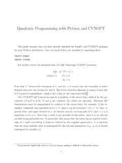
1 Basic Plotting with Python and MatplotlibThis guide assumes that you have already installed NumPy and Matplotlib for your Python can check if it is installed by importing it:import numpy as npimport as plt # The code below assumes this convenient renamingFor those of you familiar with MATLAB, the Basic Matplotlib syntax is very Line plotsThe Basic syntax for creating line plots (x,y), wherexandyare arrays of the same length thatspecify the (x, y) pairs that form the line. For example, let s plot the cosine function from 2 to 1. To doso, we need to provide a discretization (grid) of the values along thex-axis, and evaluate the function oneachxvalue.

2 This can typically be done = (-2, 1, ) # Grid of spacing from -2 to 10yvals = (xvals) # Evaluate function on (xvals, yvals) # Create line plot with yvals against () # Show the figureYou should put last after you have made all relevant changes to the plot. You cancreate multiple figures by creating new figure windows (). To output all these figures atonce, you should only have at the very end. Also, unless you turned the interactivemode on, the code will be paused until you close the figure we want to add another plot, the quadratic approximation to the cosine function.

3 We do sobelow using a different color and line type. We also add a title and axis labels, which ishighly recommendedin your own work. Also note that we moved to the end so that it shows both = 1 - * xvals**2 # Evaluate quadratic approximation on (xvals, newyvals, r-- ) # Create line plot with red dashed ( Example plots ) ( Input ) ( Function values ) () # Show the figure (remove the previous instance)The third parameter supplied is an optional format string. The particular one specifiedabove gives a red dashed line. See the extensive Matplotlib documentation online for other formattingcommands, as well as many other Plotting properties that were not covered here: # Contour plotsThe Basic syntax for creating contour plots (X,Y,Z,levels).

4 To trace a contour, a 2-D arrayZthat specifies function values on a grid. The underlying grid is given byXandY,either both as 2-D arrays with the same shape asZ, or both as 1-D arrays wherelen(X)is the number ofcolumns inZandlen(Y)is the number of rows most situations it is more convenient to work with the underlying grid ( , the former representation).Themeshgridfunction is useful for constructing 2-D grids from two 1-D arrays. It returns two 2-D arraysX,Yof the same shape, where each element-wise pair specifies an underlying (x, y) point on the grid. Functionvalues on the gridZcan then be calculated using theseX,Yelement-wise () # Create a new figure windowxlist = ( , , 100) # Create 1-D arrays for x,y dimensionsylist = ( , , 100)X,Y = (xlist, ylist) # Create 2-D grid xlist,ylist valuesZ = (X**2 + Y**2) # Compute function values on the gridWe also need to specify the contour levels (ofZ) to plot.

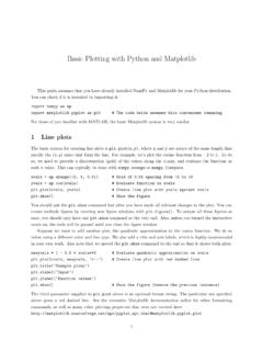
5 You can either specify a positive integer for thenumber of automatically- decided contours to plot, or you can give a list of contour (function) values in thelevelsargument. For example, we plot several contours (X, Y, Z, [ , , , ], colors = k , linestyles = solid ) ()Note that we also specified the contour colors and linestyles. By default, negative contours are given bydashed lines, hence we specifiedsolid. Again, many properties are described in the Matplotlib specification: # More Plotting propertiesThe function considered above should actually have circular contours.

6 Unfortunately, due to the differentscales of the axes, the figure likely turned out to be flattened and the contours appear like ellipses. Thisis undesirable, for example, if we wanted to visualize 2-D Gaussian covariance contours. We can force theaspect ratio to be equal with the following command (placed ) ().set_aspect( equal ) # Scale the plot size to get same aspect ratioFinally, suppose we want to zoom in on a particular region of the plot. We can do this by changing theaxis limits (again ). The input list form[xmin, xmax, ymin, ymax]. ([ , , , ]) # Set axis limitsNotice that the aspect ratio is still equal after changing the axis limits.

7 Also, the commands above onlychange the properties of the current axis. If you have multiple figures you will generally have to set themfor each figure before create the next figure can find out how to set many other axis properties at: # # final link covers many things, but most functions for changing axis properties begin with set_ .24 FiguresFigure 1: Example from section on line 2: Example from section on contour 3: Setting the aspect ratio to be equal and zooming in on the contour Codeimport numpy as npimport as pltxvals = (-2, 1, ) # Grid of spacing from -2 to 10yvals = (xvals) # Evaluate function on (xvals, yvals) # Create line plot with yvals against xvals# () # Show the figurenewyvals = 1 - * xvals**2 # Evaluate quadratic approximation on (xvals, newyvals, r-- ) # Create line plot with red dashed ( Example plots ) ( Input ) ( Function values )# () # Show the ()

8 # Create a new figure windowxlist = ( , , 100) # Create 1-D arrays for x,y dimensionsylist = ( , , 100)X,Y = (xlist, ylist) # Create 2-D grid xlist,ylist valuesZ = (X**2 + Y**2) # Compute function values on the (X, Y, Z, [ , , , ], colors = k , linestyles = solid ) ().set_aspect( equal ) # Scale the plot size to get same aspect ([ , , , ]) # Change axis ()4