Transcription of Basic Principles of Statistical Inference - Harvard University
1 Basic Principles of Statistical InferenceKosuke ImaiDepartment of PoliticsPrinceton UniversityPOL572 Quantitative Analysis IISpring 2016 Kosuke Imai (Princeton) Basic PrinciplesPOL572 Spring 20161 / 66 What is Statistics?Relatively new disciplineScientific revolution in the 20th centuryData and computing revolutions in the 21st centuryThe world is stochastic rather than deterministicProbability theory used to model stochastic eventsStatistical Inference : Learning about what we do not observe(parameters) using what we observe (data)Without statistics: wild guessWith statistics:principled guess1assumptions2formal properties3measure of uncertaintyKosuke Imai (Princeton) Basic PrinciplesPOL572 Spring 20162 / 66 Three Modes of Statistical Inference1 Descriptive Inference : summarizing and exploring dataInferring ideal points from rollcall votesInferring topics from texts and speechesInferring social networks from surveys2 Predictive Inference .
2 Forecasting out-of-sample data pointsInferring future state failures from past failuresInferring population average turnout from a sample of votersInferring individual level behavior from aggregate data3 Causal Inference : predicting counterfactualsInferring the effects of ethnic minority rule on civil war onsetInferringwhyincumbency status affects election outcomesInferring whether the lack of war among democracies can beattributed to regime typesKosuke Imai (Princeton) Basic PrinciplesPOL572 Spring 20163 / 66 Statistics for Social ScientistsQuantitative social science research:1 Find a substantive question2 Construct theory and hypothesis3 Design an empirical study and collect data4 Use statistics to analyze data and test hypothesis5 Report the resultsNo study in the social sciences is perfectUse best available methods and data, but be aware of limitationsMany wrong answers but no single right answerCredibility of data analysis:Data analysis=assumption subjective+ Statistical theory objective+interpretation subjectiveStatistical methods are no substitute for good research designKosuke Imai (Princeton) Basic PrinciplesPOL572 Spring 20164 / 66 Sample SurveysKosuke Imai (Princeton) Basic PrinciplesPOL572 Spring 20165 / 66 Sample SurveysA large population of sizeNFinite population:N< Super population:N= A simple random sample of sizenProbability sampling: , stratified, cluster, systematic samplingNon-probability sampling.
3 , quota, volunteer, snowball samplingThe population:Xifori=1,..,NSampling (binary) indicator:Z1,..,ZNAssumption: Ni=1Zi=nand Pr(Zi=1) =n/Nfor alli# of combinations:(Nn)=N!n!(N n)!Estimand=population mean vs. Estimator=sample mean:X=1NN i=1 Xiand x=1nN i=1 ZiXiKosuke Imai (Princeton) Basic PrinciplesPOL572 Spring 20166 / 66 Estimation of Population MeanDesign-based inferenceKey idea: Randomness comes from sampling aloneUnbiasedness (over repeated sampling):E( x) =XVariance of sampling distribution:V( x) =(1 nN) finite population correctionS2nwhereS2= Ni=1(Xi X)2/(N 1)is the population varianceUnbiased estimator of the variance: 2 (1 nN)s2nandE( 2) =V( x)wheres2= Ni=1Zi(Xi x)2/(n 1)is the sample variancePlug-in (sample analogue) principleKosuke Imai (Princeton) Basic PrinciplesPOL572 Spring 20167 / 66 Some VERY Important Identities in Statistics1V(X) =E(X2) {E(X)}22 Cov(X,Y) =E(XY) E(X)E(Y)3 Law of Iterated Expectation:E(X) =E{E(X|Y)}4 Law of Total Variance.
4 V(X) =E{V(X|Y)} within group variance+V{E(X|Y)} between group variance5 Mean Squared Error Decomposition:E{( )2}={E( )}2 bias2+V( ) varianceKosuke Imai (Princeton) Basic PrinciplesPOL572 Spring 20168 / 66 Analytical Details of Randomization Inference1E(Zi) =E(Z2i) =n/NandV(Zi) =E(Z2i) E(Zi)2=nN(1 nN)2E(ZiZj) =E(Zi|Zj=1)Pr(Zj=1) =n(n 1)N(N 1)fori6=jand thusCov(Zi,Zj) =E(ZiZj) E(Zi)E(Zj) = nN(N 1)(1 nN)3 Use these results to derive the expression:V( x)=1n2V(N i=1 ZiXi)=1n2 N i=1X2iV(Zi) +N i=1N j6=iXiXjCov(Zi,Zj) =1n(1 nN)1N(N 1) NN i=1X2i (N i=1Xi)2 =S2where we used the equality Ni=1(Xi X)2= Ni=1X2i NX2 Kosuke Imai (Princeton) Basic PrinciplesPOL572 Spring 20169 / 664 Finally, we proceed as follows:E{N i=1Zi(Xi x)2}=E N i=1Zi (Xi X) + (X x) add&subtract 2 =E{N i=1Zi(Xi X)2 n(X x)2}=E{N i=1Zi(Xi X)2} nV( x)=n(N 1)NS2 (1 nN)S2= (n 1)S2 Thus,E(s2) =S2, implying that the sample variance is unbiasedfor the population varianceKosuke Imai (Princeton) Basic PrinciplesPOL572 Spring 201610 / 66 Inverse Probability WeightingUnequal sampling probability: Pr(Zi=1) = ifor eachiWe still randomly samplenunits from the population of sizeNwhere Ni=1Zi=nimplying Ni=1 i=nOversampling of minorities, difficult-to-reach individuals, weights=inverse of sampling probabilityHorvitz-Thompson estimator: x=1NN i=1 ZiXi iUnbiasedness:E( x) =XDesign-based variance is complicated but availableH yek estimator (biased but possibly more efficient).
5 X = Ni=1 ZiXi/ i Ni=1Zi/ iUnknow sampling probability post-stratificationKosuke Imai (Princeton) Basic PrinciplesPOL572 Spring 201611 / 66 Model-Based InferenceAn infinite population characterized by a probabilitymodelNonparametricFParametric F ( ,N( , 2))A simple random sample of sizen:X1,..,XnAssumption:Xiis independently and identically distributed ( )according toFEstimator=sample mean vs. Estimand=population mean: 1nn i=1 Xiand E(Xi)Unbiasedness:E( ) = Variance and its unbiased estimator:V( ) = 2nand 2 1n 1n i=1(Xi )2where 2=V(Xi)Kosuke Imai (Princeton) Basic PrinciplesPOL572 Spring 201612 / 66(Weak) Law of Large Numbers (LLN)If{Xi}ni=1is a sequence of random variables with mean andfinite variance 2, thenXnp where p denotes the convergence in probability, , ifXnp x, thenlimn Pr(|Xn x|> ) =0for any >0 IfXnp x, then for any continuous functionf( ), we havef(Xn)p f(x)Implication.
6 Justifies the plug-in (sample analogue) principleKosuke Imai (Princeton) Basic PrinciplesPOL572 Spring 201613 / 66 LLN in ActionInJournal of Theoretical Biology,1 Big and Tall Parents have More Sons (2005)2 Engineers Have More Sons, Nurses Have More Daughters (2005)3 Violent Men Have More Sons (2006)4 Beautiful Parents Have More Daughters (2007)314 American Scientist, Volume 97 2009 Sigma Xi, The Scientific Research Society. Reproduction with permission only. Contact data are available for download at ~gelman/research/beautiful/As of 2007, the 50 most beautiful people of 1995 had 32 girls and 24 boys, or percent girls, which is percentage points higher than the population frequency of percent. This sounds like good news for the hypothesis. But the standard error is (32 + 24) = percent, so the discrepancy is not statistically significant.
7 Let s get more data. The 50 most beautiful people of 1996 had 45 girls and 35 boys: percent girls, or percent more than in the general population. Good news! Combining with 1995 yields percent girls percent more than expected with a stan-dard error of percent, tantaliz-ingly close to Statistical significance. Let s continue to get some confirm-ing evidence. The 50 most beautiful people of 1997 had 24 girls and 35 boys no, this goes in the wrong direction, let s keep 1998, we have 21 girls and 25 boys, for 1999 we have 23 girls and 30 boys, and the class of 2000 has had 29 girls and 25 boys. Putting all the years together and removing the duplicates, such as Brad Pitt, People s most beautiful people from 1995 to 2000 have had 157 girls out of 329 children, or percent girls (with a standard error of percent), a statistically insig-nificant percentage points lower than the population frequency.
8 So nothing much seems to be going on here. But if statistically insignificant effects were considered acceptable, we could publish a paper every two years with the data from the latest most beautiful people. Why Is This Important?Why does this matter? Why are we wasting our time on a series of pa-pers with Statistical errors that hap-pen not to have been noticed by a journal s reviewers? We have two reasons: First, as discussed in the next section, the Statistical difficul-ties arise more generally with find-ings that are suggestive but not sta-tistically significant. Second, as we discuss presently, the structure of scientific publication and media at-tention seem to have a biasing effect on social science research. Before reaching Psychology Today and book publication, Kanazawa s findings received broad attention in the news media.
9 For example, the popular Freakonomics blog reported,A new study by Satoshi Kanaza-wa, an evolutionary psychologist at the London School of Econom-ics, suggests .. there are more beautiful women in the world than there are handsome men. Why? Kanazawa argues it s be-cause good-looking parents are 36 percent more likely to have a baby daughter as their first child than a baby son which suggests, evolutionarily speaking, that beauty is a trait more valuable for women than for men. The study was conducted with data from 3,000 Americans, derived from the National Longitudinal Study of Adolescent Health, and was published in the Journal of Theo-retical in a peer-reviewed jour-nal seemed to have removed all skepti-cism, which is noteworthy given that the authors of Freakonomics are them-selves well qualified to judge social science research.
10 In addition, the estimated effect grew during the reporting. As noted above, the percent (and not sta-tistically significant) difference in the data became 8 percent in Kanazawa s choice of the largest comparison (most attractive group versus the average of the four least attractive groups), which then became 26 percent when reported as a logistic regression coefficient, and then jumped to 36 percent for reasons unknown (possibly a typo in a news-paper report). The funny thing is that the reported 36 percent signaled to us right away that something was wrong, since it was 10 to 100 times larger than reported sex-ratio effects in the bio-logical literature. Our reaction when seeing such large estimates was not Wow, they ve found something big! but, rather, Wow, this study is under-powered! Statistical power refers to the probability that a study will find a statistically significant effect if one is actually present.