Transcription of Boltzmann Transport - Physics Courses
1 Chapter 1 Boltzmann References H. Smith and H. H. Jensen, Transport Phenomena N. W. Ashcroft and N. D. Mermin,Solid State Physics , chapter 13. P. L. Taylor and O. Heinonen,Condensed Matter Physics , chapter 8. J. M. Ziman, Principles of the Theory of Solids, chapter IntroductionTransport is the phenomenon of currents flowing in response to applied fields. By current we generally mean an electrical currentj, or thermal currentjq. By applied field wegenerally mean an electric fieldEor a temperature gradient T. The currents and fieldsare linearly related, and it will be our goal to calculate the coefficients (known as transportcoefficients) of these linear relations. Implicit in our discussion is the assumption that weare always dealing with systems near 1. Boltzmann Boltzmann Equation in Semiclassical Dynamics and distribution FunctionsThe semiclassical dynamics of a wavepacket in a solid are described by the equationsdrdt=vn(k) =1~ n(k) k( )dkdt= e~E(r,t) e~cvn(k) B(r,t).
2 ( )Here,nis the band index and n(k) is the dispersion relation for bandn. The wavevectorisk(~kis the crystal momentum ), and n(k) is periodic underk k+G, whereGisany reciprocal lattice vector. These formulae are valid only at sufficiently weak fields. Theyneglect, for example, Zener tunneling processes in which an electron may change its bandindex as it traverses the Brillouin zone. We also neglect the spin-orbit interaction in are of course interested in more than just a single electron, hence to that end let usconsider the distribution functionfn(r,k,t), defined such that1fn (r,k,t)d3rd3k(2 )3 # of electrons of spin in bandnwith positions withind3rofrand wavevectors withind3kofkat timet.( )Note that the distribution function is dimensionless. By performing integrals over thedistribution function, we can obtain various physical quantities. For example, the currentdensity atris given byj(r,t) = e n, d3k(2 )3fn (r,k,t)vn(k).
3 ( )The symbol in the above formula is to remind us that the wavevector integral is performedonly over the first Brillouin now ask how the distribution functionsfn (r,k,t) evolve in time. To simplify matters,we will consider a single band and drop the indicesn . It is clear that in the absence ofcollisions, the distribution function must satisfy the continuity equation, f t+ (uf) = 0.( )This is just the condition of number conservation for electrons. Take care to note that anduaresix-dimensionalphase spacevectors:u= ( x , y , z , kx, ky, kz)( ) =( x, y, z, kx, ky, kz).( )1We will assume three space dimensions. The discussion may be generalized to quasi-two dimensionaland quasi-one dimensional systems as Boltzmann EQUATION IN SOLIDS3 Now note that as a consequence of the dynamics ( , ) that u= 0, spaceflow isincompressible, provided that (k) is a function ofkalone, and not ofr. Thus, inthe absence of collisions, we have f t+u f= 0.
4 ( )The differential operatorDt t+u is sometimes called the convective derivative .EXERCISE: Show that u= we must consider the effect of collisions, which are not accounted for by the semi-classical dynamics. In a collision process, an electron with wavevectorkand one withwavevectork can instantaneously convert into a pair with wavevectorsk+qandk q(modulo a reciprocal lattice vectorG), whereqis the wavevector transfer. Note that thetotal wavevector is preserved (modG). This means thatDtf6= 0. Rather, we should write f t+ r f r+ k f k=( f t)coll Ik{f}( )where the right side is known as thecollision integral. The collision integral is in generalafunctionofr,k, andtand afunctionalof the distributionf. As thek-dependence isthe most important for our concerns, we will writeIkin order to make this dependenceexplicit. Some examples should help clarify the , let s consider a very simple model of the collision integral,Ik{f}= f(r,k,t) f0(r,k) ( (k)).
5 ( )This model is known as therelaxation time approximation. Here,f0(r,k) is a static dis-tribution function which describes alocal equilibriumatr. The quantity ( (k)) is therelaxation time, which we allow to be energy-dependent. Note that the collision integral in-deed depends on the variables (r,k,t), and has a particularly simple functional dependenceon the more sophisticated model might invoke Fermi s golden rule, Consider elastic scatteringfrom a static potentialU(r) which induces transitions between different momentum can then writeIk{f}=2 ~ k | k U k |2(fk fk) ( k k )( )=2 ~V d3k (2 )3| U(k k )|2(fk fk) ( k k )( )where we abbreviatefk f(r,k,t). In deriving the last line we ve used plane wave wave-4 CHAPTER 1. Boltzmann Transport functions2 k(r) = exp(ik r)/ V, as well as the result k A(k) =V d3k(2 )3A(k)( )for smooth functionsA(k). Note the factor ofV 1in front of the integral in eqn. this tells us is that for a bounded localized potentialU(r), the contribution to thecollision integral is inversely proportional to the size of the system.
6 This makes sensebecause the number of electrons scales asVbut the potential is only appreciable over aregion of volume V0. Later on, we shall consider a finite density of scatterers, writingU(r) = Nimpi=1U(r Ri), where the impurity densitynimp=Nimp/Vis finite, scaling asV0. In this case U(k k ) apparently scales asV, which would meanIk{f}scales asV,which is unphysical. As we shall see, the random positioning of the impurities means thattheO(V2) contribution to| U(k k )|2isincoherentand averages out to zero. The coherentpiece scales asV, canceling theVin the denominator of eqn. , resulting in a finite valuefor the collision integral in the thermodynamic limit ( infinite nor infinitesimal).Later on we will discuss electron-phonon scattering, which isinelastic. An electron withwavevectork can scatter into a state with wavevectork=k qmodGby absorption ofa phonon of wavevectorqor emission of a phonon of wavevector q. Similarly, an electronof wavevectorkcan scatter into the statek by emission of a phonon of wavevector qorabsorption of a phonon of wavevectorq.
7 The matrix element for these processes dependsonk,k , and the polarization index of the phonon. Overall, energy is conserved. Theseconsiderations lead us to the following collision integral:Ik{f,n}=2 ~V k , |g (k,k )|2{(1 fk)fk (1 +nq, ) ( k+~ q k )+(1 fk)fk n q ( k ~ q k ) fk(1 fk ) (1 +n q ) ( k ~ q k ) fk(1 fk )nq ( k+~ q k )} q,k kmodG,( )which is a functional of both the electron distributionfkas well as the phonon distributionnq . The four terms inside the curly brackets correspond, respectively, to cases (a) through(d) in fig. collisions will violate crystal momentum conservation, they do not violate conserva-tion of particle number. Hence we should have3 d3r d3k(2 )3Ik{f}= 0.( )2 Rather than plane waves, we should use Bloch waves nk(r) = exp(ik r)unk(r), where cell functionunk(r) satisfiesunk(r+R) =unk(r), whereRis any direct lattice vector. Plane waves do not containthe cell functions, although they do exhibit Bloch periodicity nk(r+R) = exp(ik R) nk(r).
8 3If collisions are purely local, thenR d3k(2 )3Ik{f}= 0 at every pointrin Boltzmann EQUATION IN SOLIDS5 Figure : Electron-phonon total particle number,N= d3r d3k(2 )3f(r,k,t)( )is acollisional invariant- a quantity which is preserved in the collision process. Othercollisional invariants include energy (when all sources are accounted for), spin (total spin),and crystal momentum (if there is no breaking of lattice translation symmetry)4. Considera functionF(r,k) of position and wavevector. Its average value is F(t) = d3r d3k(2 )3F(r,k)f(r,k,t).( )Taking the time derivative,d Fdt= F t= d3r d3k(2 )3F(r,k){ r ( rf) k ( kf) +Ik{f}}= d3r d3k(2 )3{[ F r drdt+ F k dkdt]f+FIk{f}}.( )4 Note that the relaxation time approximation violates all such conservation laws. Within the relaxationtime approximation, there are no collisional 1. Boltzmann TRANSPORTH ence, ifFis preserved by the dynamics between collisions, thend Fdt= d3r d3k(2 )3 FIk{f},( )which says that F(t) changes only as a result of collisions.
9 IfFis a collisional invariant,then F= 0. This is the case whenF= 1, in which case Fis the total number of particles,or whenF= (k), in which case Fis the total Local EquilibriumThe equilibrium Fermi distribution ,f0(k) ={exp( (k) kBT)+ 1} 1( )is a space-independent and time-independent solution to the Boltzmann equation. Sincecollisions actlocallyin space, they act on short time scales to establish alocal equilibriumdescribed by a distribution functionf0(r,k,t) ={exp( (k) (r,t)kBT(r,t))+ 1} 1( )This is, however, not a solution to the full Boltzmann equation due to the streaming terms r r+ k kin the convective derivative. These, though, act on longer time scales thanthose responsible for the establishment of local equilibrium. To obtain a solution, we writef(r,k,t) =f0(r,k,t) + f(r,k,t)( )and solve for the deviation f(r,k,t). We will assume = (r) andT=T(r) are time-independent. We first compute the differential off0,df0=kBT f0 d( kBT)=kBT f0 { d kBT ( )dTkBT2+d kBT}= f0 { r dr+ T T r dr k dk},( )from which we read off f0 r={ r+ T T r}( f0 )( ) f0 k=~v f0.
10 ( ) CONDUCTIVITY OF NORMAL METALS7We thereby obtain f t+v f e~[E+1cv B] f k+v [eE+ T T]( f0 )=Ik{f0+ f}( )whereE= ( /e) is the gradient of the electrochemical potential ; we ll henceforthrefer toEas the electric field. Eqn ( ) is a nonlinear integrodifferential equation in f,with the nonlinearity coming from the collision integral. (In some cases, such as impurityscattering, the collision integral may be a linear functional.) We will solve alinearizedversion of this equation, assuming the system is always close to a state of local that the inhomogeneous term in ( ) involves the electric field and the temperaturegradient T. This means that fis proportional to these quantities, and if they are smallthen fis small. The gradient of fis then of second order in smallness, since the externalfields /eandTare assumed to be slowly varying in space. To lowest order in smallness,then, we obtain the followinglinearized Boltzmann equation: f t e~cv B f k+v [eE+ T T]( f0 )=L f( )whereL fis thelinearized collision integral;Lis a linear operator acting on f(we suppressdenoting thekdependence ofL).