Transcription of Calculus Online Textbook Chapter 1 - MIT OpenCourseWare
1 Chapter 1 Chapter 2 Chapter 3 Contents Introduction to Calculus Velocity and distance Calculus Without Limits The Velocity at an Instant Circular Motion A Review of Trigonometry A Thousand Points of Light Computing in Calculus Derivatives The Derivative of a Function Powers and Polynomials The Slope and the Tangent Line Derivative of the Sine and Cosine The Product and Quotient and Power Rules Limits Continuous Functions Applications of the Derivative Linear Approximation Maximum and Minimum Problems Second Derivatives: Minimum vs. Maximum Graphs Ellipses, Parabolas, and Hyperbolas Iterations x,+ ,= F(x,) Newton's Method and Chaos The Mean Value Theorem and l'H8pital's Rule Chapter 1 Introduction to Calculus Velocity and distance The right way to begin a Calculus book is with Calculus . This Chapter will jump directly into the two problems that the subject was invented to solve. You will see what the questions are, and you will see an important part of the answer.
2 There are plenty of good things left for the other chapters, so why not get started? The book begins with an example that is familiar to everybody who drives a car. It is Calculus in action-the driver sees it happening. The example is the relation between the speedometer and the odometer. One measures the speed (or velocity); the other measures the distance traveled . We will write v for the velocity, and f for how far the car has gone. The two instruments sit together on the dashboard: Fig. Velocity v and total distance f (at one instant of time). Notice that the units of measurement are different for v and distance f is measured in kilometers or miles (it is easier to say miles). The velocity v is measured in km/hr or miles per hour. A unit of time enters the velocity but not the distance . Every formula to compute v from f will have f divided by time. The central question of Calculus is the relation between v and f. --- 1 Introduction to Calculus Can you find v if you know f, and vice versa, and how?
3 If we know the velocity over the whole history of the car, we should be able to compute the total distance traveled . In other words, if the speedometer record is complete but the odometer is missing, its information could be recovered. One way to do it (without Calculus ) is to put in a new odometer and drive the car all over again at the right speeds. That seems like a hard way; Calculus may be easier. But the point is that the information is there. If we know everything about v, there must be a method to find f. What happens in the opposite direction, when f is known? If you have a complete record of distance , could you recover the complete velocity? In principle you could drive the car, repeat the history, and read off the speed. Again there must be a better way. The whole subject of Calculus is built on the relation between u and f. The question we are raising here is not some kind of joke, after which the book will get serious and the mathematics will get started.
4 On the contrary, I am serious now-and the mathematics has already started. We need to know how to find the velocity from a record of the distance . (That is called &@erentiation, and it is the central idea of dflerential Calculus .) We also want to compute the distance from a history of the velocity. (That is integration, and it is the goal of integral Calculus .) Differentiation goes from f to v; integration goes from v to f. We look first at examples in which these pairs can be computed and understood. CONSTANT VELOCITY Suppose the velocity is fixed at v =60 (miles per hour). Then f increases at this constant rate. After two hours the distance is f =120 (miles). After four hours f =240 and after t hours f =60t. We say that f increases linearly with time-its graph is a straight line. 4 velocity v(t) 4 distancef(t) v 240~~s1~="=604 Area 240 : I time t time t Fig. Constant velocity v =60 and linearly increasing distance f=60t.
5 Notice that this example starts the car at full velocity. No time is spent picking up speed. (The velocity is a "step function.") Notice also that the distance starts at zero; the car is new. Those decisions make the graphs of v and f as neat as possible. One is the horizontal line v =60. The other is the sloping line f =60t. This v, f, t relation needs algebra but not Calculus : if v is constant and f starts at zero then f =vt. The opposite is also true. When f increases linearly, v is constant. The division by time gives the slope. The distance is fl =120 miles when the time is t1 =2 hours. Later f' =240 at t, =4. At both points, the ratio f/t is 60 miles/hour. Geometrically, the velocity is the slope of the distance graph: change in distance -vtslope = in time t -- Velocity and distance Fig. Straight lines f = 20 + 60t (slope 60) and f = -30t (slope -30). The slope of the f-graph gives the v-graph. Figure shows two more possibilities: 1.
6 The distance starts at 20 instead of 0. The distance formula changes from 60t to 20 + 60t. The number 20 cancels when we compute change in distance -so the slope is still 60. 2. When v is negative, the graph off goes downward. The car goes backward and the slope off = -30t is v = -30. I don't think speedometers go below zero. But driving backwards, it's not that safe to watch. If you go fast enough, Toyota says they measure "absolute valuesw-the speedometer reads + 30 when the velocity is -30. For the odometer, as far as I know it just stops. It should go VELOCITY vs. distance : SLOPE vs. AREA How do you compute f' from v? The point of the question is to see f = ut on the graphs. We want to start with the graph of v and discover the graph off. Amazingly, the opposite of slope is area. The distance f is the area under the v-graph. When v is constant, the region under the graph is a rectangle. Its height is v, its width is t, and its area is v times t.
7 This is integration, to go from v to f by computing the area. We are glimpsing two of the central facts of Calculus . 1A The slope of the f-graph gives the velocity v. The area under the v-graph gives the distance f. That is certainly not obvious, and I hesitated a long time before I wrote it down in this first section. The best way to understand it is to look first at more examples. The whole point of Calculus is to deal with velocities that are not constant, and from now on v has several values. EXAMPLE (Forward and back) There is a motion that you will understand right away. The car goes forward with velocity V, and comes back at the same speed. To say it more correctly, the velocity in the second part is -V. If the forward part lasts until t = 3, and the backward part continues to t = 6, the car will come back where it started. The total distance after both parts will be f = 0. +This actually happened in Ferris Bueller's Day 08,when the hero borrowed his father's sports car and ran up the mileage.
8 At home he raised the car and drove in reverse. I forget if it worked. 1 Introductionto Calculus 1u(r) = slope of f(t) Fig. Velocities + V and -V give motion forward and back, ending at f(6)=0. The v-graph shows velocities + V and -V. The distance starts up with slope + V and reaches f = 3V. Then the car starts backward. The distance goes down with slope -V and returns to f = 0 at t = 6. Notice what that means. The total area "under" the v-graph is zero! A negative velocity makes the distance graph go downward (negative slope). The car is moving backward. Area below the axis in the v-graph is counted as negative. FUNCTIONS This forward-back example gives practice with a crucially important idea-the con-cept of a "jiunction." We seize this golden opportunity to explain functions: The number v(t) is the value of the function t. at the time t. The time t is the input to the function. The velocity v(t) at that time is the output.
9 Most people say "v oft" when they read v(t). The number "v of 2" is the velocity when t = 2. The forward-back example has v(2) = + V and v(4) = -V. The function contains the whole history, like a memory bank that has a record of v at each t. It is simple to convert forward-back motion into a formula. Here is v(t): The ,right side contains the instructions for finding v(t). The input t is converted into the output + V or -V. The velocity v(t) depends on t. In this case the function is "di~continuo~s,~'because the needle jumps at t = 3. The velocity is not dejined at that instant. There is no v(3). (You might argue that v is zero at the jump, but that leads to trouble.) The graph off' has a corner, and we can't give its slope. The problem also involves a second function, namely the distance . The principle behind f(t) is the same: f (t) is the distance at time t. It is the net distance forward, and again the instructions change at t = 3.
10 In the forward motion, f(t) equals Vt as before. In the backward half, a calculation is built into the formula for f(t): At the switching time the right side gives two instructions (one on each line). This would be bad except that they agree: f (3)= distance function is "con- ?A function is only allowed one ~:alue,f'(r) at each time ror ~(t) Velocity and distance tinuous." There is no jump in f, even when there is a jump in v. After t = 3 the distance decreases because of -Vt. At t = 6 the second instruction correctly gives f (6) = 0. Notice something more. The functions were given by graphs before they were given by formulas. The graphs tell you f and v at every time t-sometimes more clearly than the formulas. The values f (t) and v(t) can also be given by tables or equations or a set of instructions. (In some way all functions are instructions-the function tells how to find f at time t.) Part of knowing f is knowing all its inputs and outputs-its domain and range: The domain of a function is the set of inputs.