Ch 2.7: Numerical Approximations: Euler’s Method

1 Ch : Numerical Approximations: euler s Method Recall that a first order initial value problem has the form If f and f / yare continuous, then this IVP has a unique solution y= (t) in some interval about t0. When the differential equation is linear, separable or exact, we can find the solution by symbolic manipulations. However, the solutions for most differential equations of this form cannotbe found by analytical means. Therefore it is important to be able to approach the problem in other ways. 00)(),,(ytyytfdtdy Direction Fields For the first order initial value problem (IVP)we can sketch a direction field and visualize the behavior of solutions.

2 ** This has the advantage of being a relatively simple process, even for complicated equations. ** However, direction fields do not lend themselves to quantitative computations or comparisons ( with experiment data),)(),,(00ytyytfy Numerical methods For our first order initial value probleman alternative is to compute approximate values of the solution y= (t) at a selected set oft-values. Ideally, the approximate solution values will be accompanied by errorbounds that ensure the level of accuracy. There are many Numerical methods that produce Numerical approximations to solutions of differential equations, some of which are discussed in Chapter 8.

3 In this section, we examine the tangent line Method , which is also called euler s Method . Tangent line Method : approximate the unknown solution y(t) by tangent lines,)(),,(00ytyytfy euler s Method : Tangent Line approximation For the initial value problem we begin by approximating solution y= (t) at initial point t0. The solution passes through initial point (t0, y0) with slope f(t0, y0). The line tangent to the solution at this initial point is The tangent line is a good approximation to solution curve on an interval short enough.

4 Thus if t1is close enough to t0, we can approximate (t1) by 0000,ttytfyy ,)(),,(00ytyytfy 010001,ttytfyy euler s Formula For a point t2close to t1, we approximate (t2) using the line passing through (t1, y1) with slope f(t1, y1): Thus we create a sequence ykof approximations to (tk):where fk= f(tk, yk). For a uniform step size h= tk tk-1, euler s formula becomes 100102112111kkkkkyyfttyyfttyyftt 121112,ttytfyy 1, 0,1, 2,kkkyyf hk euler approximation To graph an euler approximation , we plot the points (t0, y0), (t1, y1).

5 , (tn, yn), and then connect these points with line segments. nnnnnnnnytffttfyy, where,11 Example 1: euler s Method (1 of 3) For the initial value problem We can use euler s Method with h= to approximate the solution at t= , , , , and as shown below. ) ( ) ( ) ( ) ( ) ( ) )( (1445334223112001 hfyyhfyyhfyyhfyyhfyy1)0(, yytdtdyExample 1: Exact Solution (2 of 3) We can find the exact solution to our IVP, as in Chapter )0( )0(, files Files: , , ( ~dfield)--For using these files, Read the guideline in course main webpage: (Example) y = 2y t + 1, y(0) = 1 (How to use )(1) create M-file, (2) The syntax for eul.

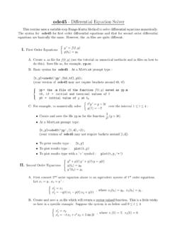
6 > eul( fcn1 ,[t0, tf],y(0),h)--t0 = the initial value of x --tf= the final value of t--y(0) = the initial value of y --h = the step size.(3) You can try > eul( fcn1 ,[0,3],1, )(4) To plot the Numerical solution we can try> [t,y] = eul( fcn1 ,[0,3],1, )> plot(t,y) You can also create your own M-files221 5()44tty te euler Method (Tangent line Method ) (Example) By using the euler Method approximate the solution of the ODE with h = : (Example) Estimate by using eul with h = (Hint) What if we set Remark: When we use these routines, things can go wrong !

7 !(1) Step size is too large or too small.(2) Solution may not be defined at point in ( )x dx 21( )sin( ) ? What is = ?tdyy tx dxdt 22, (1) Error estimateExample 1: euler s Method (1 of 3) For the initial value problemwe can use euler s Method with various step sizes (h) to approximate the solution at t= , , , , and and compare our results to the exact solutionat those values of , (0) 1dytyydt Example 1: euler s Method (2 of 3) Comparison of exact solution with euler s Method for h = , , , tExact yh = = = = 1.

8 Error Analysis (3 of 3) From table below, we see that the errors start small, but get larger. This is most likely due to the fact that the exact solution is not linear on [0, 1]. Note: tExact yApprox yError% Rel Error RelativePercent y in redApproximate y in blueExample 2: euler s Method (1 of 3) For the initial value problemwe can use euler s Method with h= to approximate the solution at t= 1, 2, 3, and 4, as shown below. Exact solution (see Chapter ): ) () )(2( ) () )(2( ) () )(2( ) ()1)(2(041334223112001 hfyyhfyyhfyyhfyy1)0(,24 yytdtdytety24112147 Example 2: Error Analysis (2 of 3) The first ten euler approxs are given in table below on left.

9 A table of approximations for t= 0, 1, 2, 3 is given on right. See text for Numerical results with h= , , The errors are small initially, but quickly reach an unacceptable level. This suggests a nonlinear solution. tExact yApprox yError% Rel yApprox yError% Rel :SolutionExact Example 2: Error Analysis & Graphs (3 of 3) Given below are graphs showing the exact solution (red) plotted together with the euler approximation (blue). tExact yApprox yError% Rel :SolutionExact General Error Analysis Discussion (1 of 4) Recall that if f and f / yare continuous, then our first order initial value problemhas a solution y= (t) in some interval about t0.

10 In fact, the equation has infinitely many solutions, each one indexed by a constant cdetermined by the initial condition. Thus is the member of an infinite family of solutions that satisfies (t0) = y0. 00)(),,(ytyytfdtdy General Error Analysis Discussion (2 of 4) The first step of euler s Method uses the tangent line to at the point (t0, y0) in order to estimate (t1) with y1. The point (t1, y1) is typically not on the graph of , because y1is an approximation of (t1). Thus the next iteration of euler s Method does not use a tangent line approximation to , but rather to a nearby solution 1that passes through the point (t1, y1).