Transcription of Chap. 5: Joint Probability Distributions
1 Chap. 5: Joint Probability Distributions Probability modeling of several RV s We often study relationships among variables. Demand on a system = sum of demands from subscribers (D = S1 + S2 + . + Sn). Surface air temperature & atmospheric CO2. Stress & strain are related to material properties; random loads; etc. Notation: Sometimes we use X1 , X2 , ., Xn Sometimes we use X, Y, Z, etc. 1. Sec : Basics First, develop for 2 RV (X and Y). Two Main Cases I. Both RV are discrete II. Both RV are continuous I. (p. 185). Joint Probability Mass Function (pmf) of X and Y is defined for all pairs (x,y) by p( x, y ) P( X x and Y y ).
2 P( X x, Y y ). 2. pmf must satisfy: p( x, y) 0 for all ( x, y). x y p( x, y) 1. for any event A, P ( X , Y ) A p( x, y). ( x , y ) A. 3. Joint Probability Table: Table presenting Joint Probability distribution : y Entries: p( x, y ) 1 2 3. P(X = 2, Y = 3) = .13 x 1 .10 .15 .22. 2 .30 .10 .13. P(Y = 3) = .22 + .13 = .35. P(Y = 2 or 3) = .15 + .10 + .35 =.60. 4. The marginal pmf X and Y are p X ( x) y p( x, y) and pY ( y) x p( x, y). y 1 2 3. x 1 .10 .15 .22 .47. 2 .30 .10 .13 .53..40 .25 .35. x 1 2 y 1 2 3. pX(x) .47 .53 pY(y) .40 .25 .35. 5. II. Both continuous (p.)
3 186). A Joint Probability density function (pdf) of X and Y is a function f(x,y) such that f(x,y) > 0 everywhere .. f ( x, y)dxdy 1. and P[( X , Y ) A] f ( x, y)dxdy A. 6. pdf f is a surface above the (x,y)-plane A is a set in the (x,y)-plane. P[( X , Y ) A] is the volume of the region over A under f. (Note: It is not the area of A.). f y x A. 7. Ex) X and Y have Joint PDF. f(x,y) = c x y2 if 0 < x < y < 1. = 0 elsewhere. Find c. First, draw the region where f > 0. 1 y 1. 1 cxy2. dxdy . y 0 0 0 1. 1 1. x cxy2. dydx 1 y cxy 2. 0 x (not dxdy x 0. 1 y 1 1.
4 Dy c / 10. 2 2 2 y 4. cxy dxdy c y [.5 x | 0 ]dy c .5 y 0 0 0 0. so, c = 10 1. Find P(X+Y<1). y First, add graph of x + y =1. 0 1..5 y 1 1 y x P( X Y 1) .. 10 xy 2. dxdy 10 xy 2. dxdy 0 0 .5 0..5 1 x 1 x .5. y 3. x 10 xy dydx 10 0 x 3 dx . 2. 0 x .5. (10 / 3) x((1 x) 3 x 3 )dx .135. 0. Marginal pdf (p. 188) . Marginal pdf of X: f X ( x) f ( x, y)dy .. Marginal pdf of Y: fY ( y ) .. f ( x, y)dx Ex) X and Y have Joint PDF. f(x,y) = 10 x y2 if 0 < x < y < 1 , and 0 else. For 0 < y < 1: y y fY ( y ) f ( x, y)dx 10 xy dx 10 y xdx 5 y 2 2 4. 0 0. and fY ( y) 0 otherwise.
5 10. marginal pdf of Y: fY ( y) 5 y for 0 y 1 and is 0 otherwise. 4. marginal pdf of Y: you check f X ( x) (10 / 3) x(1 x ) for 0 x 1. 3. Notes: and is 0 otherwise. 1. x cannot appear in fY ( y ) (y can t be in f X (x) ). 2. You must give the ranges; writing fY ( y) 5 y 4. is not enough. Math convention: writing Y f ( y ) 5 y 4. with no range means it s right for all y, which is very wrong in this example. 11. Remark: distribution Functions For any pair of jointly distributed RV, the Joint distribution function (cdf) of X and Y. is F ( x, y) P( X x, Y y).
6 Defined for all (x,y). For X,Y are both continuous: 2. f ( x, y ) F ( x, y ). x y wherever the derivative exists. 12. Extensions for 3 or more RV: by example X, Y, Z are discrete RV with Joint pmf p( x, y, z) P( X x, Y y, Z z). marginal pmf of X is p X ( x) y z p( x, y, z ) (= P(X = x)). ( Joint ) marginal pmf of X and Y is p XY ( x, y) z p( x, y, z ) (= P(X=x, Y = y)). 13. X, Y, Z are continuous RV with Joint pdf f(x,y,z): marginal pdf of X is . f X ( x) f ( x, y, z )dydz . ( Joint ) marginal pmf of X and Y is . f XY ( x, y ) f ( x, y, z )dz . 14. Conditional Distributions & Independence.
7 Marginal pdf of X: f X ( x) f ( x, y )dy . Marginal pdf of Y: . fY ( y ) f ( x, y)dx . Conditional pdf of X. given Y=y (h(y) > 0) f ( x | y) f ( x, y) / h( y). Conditional prob P( X A | Y y) f ( x | y)dx for X for y fixed A. 15. Conditional Distributions & Independence Review from Chap. 2: For events A & B where P(B) > 0, define P(A|B). to be the conditional prob. that A occurs given B occurred: P(A | B)=P(A I B) / P(B). Multiplication Rule: P(A I B) = P(A) P(B|A). = P(B) P(A|B). Events A and B are independent if P(B|A) = P(B). or equivalently P(A I B) = P(A) P(B).
8 Extensions to RV. Again, first, develop for 2 RV (X and Y). Two Main Cases I. Both RV are discrete II. Both RV are continuous I. (p. 193). Conditional Probability Mass Function (pmf) of Y given X = x is p( x, y ) Joint pY | X ( y | x) . p X ( x) marginal of condition as long as p X ( x) 0. 17. Note that idea is the same as in Chap. 2. P( X x, Y y ). P(Y y | X x) . P( X x). as long as P( X x) 0. However, keep in mind that we are defining a (conditional) prob. dist for Y for a fixed x 18. Example: y x 1 2. 1 2 3 pX(x) .47 .53. x 1 .10 .15 .22 .47. y 1 2 3.
9 2 .30 .10 .13 .53..40 .25 .35 pY(y) .40 .25 .35. Find cond l pmf of X given Y = 2: p( x, y ) gives p ( x | 2) p( x,2). p X |Y ( x | y ) X |Y. pY ( y ) pY (2). So x 1 2. pX|Y(x|2) .15/.25=.60 .10/.25=.40. 19. II. Both RV are continuous (p. 193). Conditional Probability Density Function (pdf) of Y given X = x is f ( x, y) Joint pdf f Y | X ( y | x) . f X ( x) marginal pdf of condition as long as f X ( x) 0. The point: P(Y A | X x) fY | X ( y | x)dy A. 20. Remarks ALWAYS: for a cont. RV, prob it s in a set A is the integral of its pdf over A: no conditional; use the marginal pdf with a condition; use the right cond l pdf Interpretation: For cont.
10 X, P(X = x) = 0, so by Chap 2 rules, P(Y A | X x) is meaningless. There is a lot of theory that makes sense of this For our purposes, think of it as an approximation to P(Y A | X x). that is given X lies in a tiny interval around x . 21. Ex) X, Y have pdf f(x,y) = 10 x y2 if 0 < x < y < 1 , and = 0 else. Conditional pdf of X given Y= y: f X |Y ( x | y) f ( x, y) / fY ( y). We found fY(y) = 5y4 for 0<y<1, = 0 else. So 2. 10 xy f ( x | y) 4. if 0 < x < y < 1. 5y Final Answer: For a fixed y, 0 < y < 1, fX|Y(x | y) = 2x / y2 if 0 < x < y, and = 0 else.