Chapter 10.02 Parabolic Partial Differential Equations

1 Chapter Parabolic Partial Differential Equations After reading this Chapter , you should be able to: 1. Use numerical methods to solve Parabolic Partial Differential Equations by explicit, implicit, and Crank-Nicolson methods. The general second order linear PDE with two independent variables and one dependent variable is given by 022222=+ + + DyuCyxuBxuA (1) where CBA,,are functions of the independent variables, x ,y, and D can be a function of xuuyx ,,, and yu.

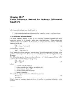
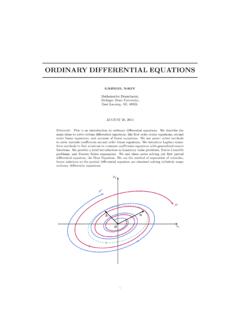
2 If 042= ACB, Equation (1) is called a Parabolic Partial Differential equation. One of the simple examples of a Parabolic PDE is the heat-conduction equation for a metal rod (Figure 1) tTxT = 22 (2) where =T temperature as a function of location, x and time, t in which the thermal diffusivity, is given by Ck = where =kthermal conductivity of rod material, = density of rod material, =C specific heat of the rod material. Chapter Figure 1: A metal rod Explicit Method of Solving Parabolic PDEs To numerically solve Parabolic PDEs such as Equation (2), one can use finite difference approximations of the Partial derivatives so that the dependent variable, T is now sought at particular nodes (x-location) and time (t) (Figure 2).

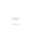
3 The left hand side second derivative is approximated by the central divided difference approximation as ( )211,222xTTTxTjijijiji + + (3) where =inode number along the xdirection, ni,..,1,0=, j= node number along the time, x = distance between nodes. Figure 2: Schematic diagram showing the node representation in the model For a rod of length L which is divided into 1+n nodes, nLx= (4) The time is similarly broken into time steps of t.

4 Hence jiT corresponds to the temperature at node i, that is, ( )( )xix = and time, ( )( )tjt =, where = ttime step. x1 ii1+ix x Parabolic Partial Differential Equations The time derivative of the right hand side of Equation (2) is approximated by the forward divided difference approximation tTTtTjijiji +1, (5) Substituting the finite difference approximations given by Equations (3) and (5) in Equation (2) gives ( )tTTxTTTjijijijiji = + + +12112 Solving for the temperature at the time node1+j, gives ()

5 JijijijijiTTTxtTT11212)( +++ += Choosing 2)(xt = (6) ()jijijijijiTTTTT1112 +++ += (7) Equation (7) can be solved explicitly because it can be written for each internal location node of the rod for time node 1+j in terms of the temperature at time node j. In other words, if we know the temperature at node0=j, and knowing the boundary temperatures, which is the temperature at the external nodes, we can find the temperature at the next time step.

6 We continue the process by first finding the temperature at all nodes 1=j, and using these to find the temperature at the next time node, 2=j. This process continues till we reach the time at which we are interested in finding the temperature. Example 1 A rod of steel is subjected to a temperature of C 100 on the left end and C 25 on the right end. If the rod is of , use the explicit method to find the temperature distribution in the rod from 0=tand 9=tseconds. , st3= . Given: KmWk =54, 37800mkg= , KkgJC =490. The initial temperature of the rod isC 20.

7 Solution Ck = 490780054 = = Then ( )2xt = Chapter ( ) = Number of time steps=tttinitialfinal 309 = 3= Figure 3: Schematic diagram showing the node distribution in the rod The boundary conditions 3,2,1,0allfor2510050= = =jCTCTjj ( ) The initial temperature of the rod is C 20, that is, all the temperatures of the nodes inside the rod are at C 20 when time, sec0=t except for the boundary nodes as given by Equation ( ).

8 This could be represented as 1,2,3,4 allfor ,200= =iCTi. ( ) Initial temperature at the nodes inside the rod (when t=0 sec) ( )Equationfrom10000CT = ( )Equationfrom2020202004030201 = = = =CTCTCTCT ( )Equationfrom2505CT = Temperature at the nodes inside the rod when t=3 sec Setting 0=j and 5,4,3,2,1,0=i in Equation (7) gives the temperature of the nodes inside the rod when time, sec3=t. 0= =25CT =100 Parabolic Partial Differential Equations ( )ConditionBoundary10010CT = ()()( )CTTTTT =+=+=+ +=+ += )20( ()()( )CTTTTT =+=+=+ +=+ += )20( ()()( )CTTTTT =+=+=+ +=+ += )20( ()()( )CTTTTT =+=+=+ +=+ += )20( ( )ConditionBoundary2515CT = Temperature at the nodes inside the rod when t=6 sec Setting 1=j and 5,4,3,2,1,0=i in Equation (7) gives the temperature of the nodes inside the rod when time, sec6=t ( )

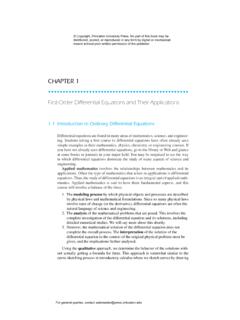
9 ConditionBoundary10020CT = Chapter ()()()CTTTTT =+=+=+ +=+ += ) ( ()()()CTTTTT =+=+=+ +=+ += )20( ()()()CTTTTT =+=+=+ +=+ += )20( ()()( )CTTTTT =+=+=+ +=+ += ) ( ( )ConditionBoundary2525CT = Temperature at the nodes inside the rod when t=9 sec Setting 2=j and 5,4,3,2,1,0=i in Equation (7) gives the temperature of the nodes inside the rod when time, sec9=t ( )ConditionBoundary10030CT = ()()()CTTTTT =+=+=+ +=+ += ) ( Parabolic Partial Differential Equations ()()()CTTTTT =+=+=+ +=+ += ) ( ()()()CTTTTT =+=+=+ +=+ += ) ( ()()()CTTTTT =+=+=+ +=+ += ) ( ( )ConditionBoundary2535CT = To better visualize the temperature variation at different locations at different times, temperature distribution along the length of the rod at different times is plotted in the Figure 4.

10 Figure 4: Temperature distribution from explicit method Chapter Implicit Method for Solving Parabolic PDEs In the explicit method, one is able to find the solution at each node, one equation at a time. However, the solution at a particular node is dependent only on temperature from neighboring nodes from the previous time step. For example, in the solution of Example 1, the temperatures at node 2 and 3 artificially stay at the initial temperature at 3=t seconds. This is contrary to what we would expect physically from the problem.