Transcription of Chapter 11 Finite element analysis
1 Applied Engineering analysis - slides for class teaching* Chapter 11 Introduction to Finite - element AnalysisChapter 11 Finite element analysis Tai-Ran Hsu on the textbook on Applied Engineering analysis by Tai-Ran Hsu, published byJohn Wiley & Sons, 2018(ISBN 9781119071204) 1 chapter Learning Objectives Learn the principle of Finite element method for engineering analyses. Learn the concept of discretization of continua for approximation solutions. Become familiar with the steps in general Finite element analysis . Learn the derivation of interpolation functions for simplex elements. Learn the variational principle in deriving element equations.
2 Learn the derivation of element equations using the Rayleigh-Ritz method and the Galerkin method. Learn the input/output in general Finite element analysis . Learn to assemble element equations to the overall stiffness equations. Learn to solve for primary unknown quantities from overall stiffness equations. Learn to relate the primary unknown quantities obtained from the Finite element method to other required secondary unknown quantities. Learn the use of general-purpose Finite element analysis codes adopted by industry in solving complex real-world problems. of Finite element Method (FEM) ( )We have emphasized the importance of Stage 2 in the 4 stages in general cases of engineering analysis in Chapter 1.
3 This stage requires engineers to idealize many physical situations in the problems that they are dealing with, so that they can use their available tools to handle the problems in the subsequent mathematical modeling, followed by the stage of interpretation of analysis results in the idealizations, though are necessary in getting the jobs done , but usually would result in compromising the required accuracies in results in many occasions. Significant safety factors need to be introduced to compensate many less than realistic idealizations made in the analysis . Many would call the safety factors that engineers often need to introduce in their analysis with a layman s term of factors of ignorance.
4 FEM was used in many concurrent engineering anlyses to alleviate the needs for engineers making less than realistic idealizations on the real physical situations. Advanced Finite element analyses offered by many commercially available general purpose codes have also been used to simulate performances of new engineering systems with established computer aided design packages. Simulation of product s performance has save significant cost and time on producing and testing of real prototypes, as well as time required to produce and testing these prototypes in traditional engineering practices. Principle of FEM ( )The essence of the Finite element method can be summarized in a simple phrase of Divide and Conquer.
5 The core strategy of the FEM is indeed to divide continua of complicated geometry with infinite number of degree of freedom(dof) in the solutions into a Finite number of sub divisions of the continua with specific simple geometry called elements. These elements are interconnected at specific points, either on the sides of the elements and/or at the corners called nodes in a discretized model. element equations are derived for each of these elements in the discretized model based on the appropriate physical theories and principles. An overall structural equation is then derived by assembling all the element equations in the discretized model, upon which the specified loading and boundary conditions on the original continuum are applied.
6 Desired solutions on the unknown quantities are solved from these overall structural equations at every element and nodes using the techniques of solving simultaneous linear equations such as the Gaussian elimination method or its derivativesas presented in Section on Because the desired solutions are made available only at the Finite number of the elements (and nodes) in the discretized model, but not everywhere in the original continuum. In other word, the Finite element method provides solutions at elements and nodes of the discretized continua. It thus has reduced the total infinite number of dofwith the original continua to a Finite number degree of freedom (dof)after they are discretized in the Finite element analysis .
7 The concept of divide and concur can thus be viewed as the fundamental principle of this method. in Finite element analysis ( )FEM is now being used in virtually every engineering disciplines, as well as in science, economics, agriculture, and even in financial institutions. It is not possible to establish a set of standard procedures for all the computations for the problems described in thee disciplines. We will focus our attention in formulations on deformable solids, as often used in mechanical engineering However, as a general guideline, most Finite elements analyses follow eight (8) steps, as will be described 1: Discretization of the real structures ( )Discretization of continua in engineering analyses is the foundation for the formulation of the Finite element analysis .
8 We will present the mathematical expressions that illustrate the principle of the Finite element method by dividing the continuum subjected to a system actions of forces, and/or heat fluxes, and/or pressures as shown in Figure (a) into a number of elements of specific geometry interconnected at the nodes (shown in black dots) in Figure (b).(a) A continuous solid(b) A discretized solidFigure Solid subjected to LoadsDiscretization56 The discretized model in Figure (b) offers an approximation in the geometry of the original continuum in Figure (a). One noticeable difference is the continuous curved boundary of the original medium is now represented by cords of straightedges in the discretized medium for the Finite element analysis .
9 Step 1: Discretization of the real structures Cont in Finite element analysis Cont d(a) A continuous solid(b) A discretized solidFigure Solid subjected to LoadsDiscretizationFigure Common shapes of elementsBar elements: for truss members and beamsPlate elements: for plane structures such as and platesTorus elements: for solids structures of axisymmetric geometry,such as cylinders and disksTetrahedron and Hexahedron elements: for solids of 3 D geometryCommon geometry of elements:7 Step 1: Discretization of the real structures Cont in Finite element analysis Cont d(a) A continuous solid(b) A discretized solidFigure Solid subjected to LoadsDiscretizationIt is important that engineers set the discretized FE model in a fixed coordinate system, such as shown in Figure (b) for a tapered plate :(a) A Tapered plate(b) Discretized tapered plate with quadrilateral and triangular plate elementsFigure FE model for a tapered bar subjected to tensile forces18 elements and 25 in Finite element analysis Cont dStep 1: Discretization of the real structures Cont d.
10 Identities of elements and nodes in discretized model:(a) A Tapered plate(b) Discretized tapered plate with quadrilateral and triangular plate elementsNode No. x coordinate y coordinateNodal constraintsApplied nodal force(cm)(cm)in displacements10 0ux= uy= 0718 0F80 3 ux= 014183F1506ux= 01766181061912421184F2208ux= node numbers Material characterized by input material number11,2,9,8166,7,14,13176,9,16,15189, 10,17,1611213,14,21,2011315,23,22,221141 5,16,23,2311516,24,23,2311616,17,24,2411 717,25,24,2411817,18,25,251 Nodal description of FE model of a tapered barElement description of FE model of a tapered barInput of nodaland elementinformation (18 elements and 25 nodes):Designation of plate deformationbynodal displacements (movements).