Transcription of Chapter 11 Pricing Strategies for Firms with Market …
1 Copyright 2010 by the McGraw-Hill Companies, Inc. All rights Economics & Business StrategyChapter 11 Pricing Strategies for Firms with Market Power11-2 OverviewI. Basic Pricing Strategies Monopoly & Monopolistic Competition Cournot OligopolyII. Extracting Consumer Surplus Price Discrimination Two-Part Pricing Block Pricing Commodity BundlingIII. Pricing for Special Cost and Demand Structures Peak-Load Pricing Transfer Pricing Cross SubsidiesIV. Pricing in Markets with Intense Price Competition Price Matching Randomized Pricing Brand Loyalty11-3 Standard Pricing and Profits for Firms with Market PowerPriceQuantityP = 10 - 2Q1086421 2 34 5 MCMR = 10 - 4 QProfits from standard Pricing = $811-4An Algebraic Example P = 10 - 2Q C(Q) = 2Q If the firm must charge a single price to all consumers, the profit-maximizing price is obtained by setting MR = MC.
2 10 - 4Q = 2, so Q* = 2. P* = 10 - 2(2) = 6. Profits = (6)(2) - 2(2) = $ Simple Markup Rule Suppose the elasticity of demand for the firm s product is EF. Since MR = P[1 + EF]/ EF. Setting MR = MC and simplifying yields this simple Pricing formula:P = [EF/(1+ EF)] MC. The optimal price is a simple markup over relevant costs! More elastic the demand, lower markup. Less elastic the demand, higher Example Elasticity of demand for Kodak film is -2. P = [EF/(1+ EF)] MC P = [-2/(1 - 2)] MC P = 2 MC Price is twice marginal cost. Fifty percent of Kodak s price is margin above manufacturing Rule for Cournot Oligopoly Homogeneous product Cournot oligopoly. N = total number of Firms in the industry. Market elasticity of demand EM . Elasticity of individual firm s demand is given by EF= N x EM. Since P = [EF/(1+ EF)] MC, Then, P = [NEM/(1+ NEM)] MC. The greater the number of Firms , the lower the profit-maximizing markup Example Homogeneous product Cournot industry, 3 Firms .
3 MC = $10. Elasticity of Market demand = - . Determine the profit-maximizing price? EF= N EM = 3 (-1/2) = P = [EF/(1+ EF)] MC. P = [ (1- ] $10. P = 3 $10 = $ Consumer Surplus: Moving From Single Price Markets Most models examined to this point involve a single equilibrium price. In reality, there are many different prices being charged in the Market . Price discrimination is the practice of charging different prices to consumer for the same good to achieve higher prices. The three basic forms of price discrimination are: First-degree (or perfect) price discrimination. Second-degree price discrimination. Third-degree price or Perfect Price Discrimination Practice of charging each consumer the maximum amount he or she will pay for each incremental unit. Permits a firm to extract all surplus from Price DiscriminationPriceQuantityD1086421 2 3 4 5 Profits*.)
4 5(4-0)(10 - 2)= $16 Total Cost* = $8MC* Assuming no fixed costs11-12 Caveats: In practice, transactions costs and information constraints make this difficult to implement perfectly (but car dealers and some professionals come close). Price discrimination won t work if consumers can resell the Price Discrimination The practice of posting a discrete schedule of declining prices for different quantities. Eliminates the information constraint present in first-degree price discrimination. Example: Electric utilitiesPriceMCD$5$104 Quantity$8211-14 Third-Degree Price Discrimination The practice of charging different groups of consumers different prices for the same product. Group must have observable characteristics for third-degree price discrimination to work. Examples include student discounts, senior citizen s discounts, regional & international Third-Degree Price Discrimination Suppose the total demand for a product is comprised of two groups with different elasticities, E1< E2.
5 Notice that group 1 is more price sensitive than group 2. Profit-maximizing prices? P1= [E1/(1+ E1)] MC P2 = [E2/(1+ E2)] MC11-16An Example Suppose the elasticity of demand for Kodak film in the US is EU= , and the elasticity of demand in Japan is EJ= Marginal cost of manufacturing film is $3. PU= [EU/(1+ EU)] MC = [ (1 - )] $3 = $9 PJ= [EJ/(1+ EJ)] MC = [ (1 - )] $3 = $5 Kodak s optimal third-degree Pricing strategy is to charge a higher price in the US, where demand is less Pricing When it isn t feasible to charge different prices for different units sold, but demand information is known, two-part Pricing may permit you to extract all surplus from consumers. Two-part Pricing consists of a fixed fee and a per unit charge. Example: Athletic club Two-Part Pricing Works1. Set price at marginal Compute consumer Charge a fixed-fee equal to consumer 2 34 5 MCFixed Fee = Profits* = $16 PricePer UnitCharge* Assuming no fixed costs11-19 Block Pricing The practice of packaging multiple units of an identical product together and selling them as one package.
6 Examples Paper. Six-packs of soda. Different sized of cans of green Algebraic Example Typical consumer s demand is P = 10 - 2Q C(Q) = 2Q Optimal number of units in a package? Optimal package price?11-21 Optimal Quantity To Package: 4 UnitsPriceQuantityD1086421 2 34 5MC = AC 11-22 Optimal Price for the Package: $24 PriceQuantityD1086421 2 34 5MC = ACConsumer s valuation of 4units = .5(8)(4) + (2)(4) = $24 Therefore, set P = $24!11-23 Costs and Profits with Block PricingPriceQuantityD1086421 2 34 5MC = ACProfits* = [.5(8)(4) + (2)(4)] (2)(4)= $16 Costs = (2)(4) = $8* Assuming no fixed costs11-24 Commodity Bundling The practice of bundling two or more products together and charging one price for the bundle. Examples Vacation packages. Computers and software. Film and Example that Illustrates Kodak s Moment Total Market size for film and developing is 4 million consumers.
7 Four types of consumers 25% will use only Kodak film (F). 25% will use only Kodak developing (D). 25% will use only Kodak film and use only Kodak developing (FD). 25% have no preference (N). Zero costs (for simplicity). Maximum price each type of consumer will pay is as follows:11-26 Reservation Prices for Kodak Film and Developing by Type of ConsumerTypeFilm DevelopingF$8$3FD$8$4D$4$6N$3$211-27 Optimal Film Price?TypeFilm DevelopingF$8$3FD$8$4D$4$6N$3$2 Optimal Price is $8; only types F and FD buy resulting in profits of $8 x 2 million = $16 a price of $4, only types F, FD, and D will buy (profits of $12 Million).At a price of $3, all will types will buy (profits of $12 Million).11-28 Optimal Price for Developing?TypeFilm DevelopingF$8$3FD$8$4D$4$6N$3$2 Optimal Price is $3, to earn profits of $3 x 3 million = $9 a price of $6, only D type buys (profits of $6 Million).
8 At a price of $4, only D and FD types buy (profits of $8 Million).At a price of $2, all types buy (profits of $8 Million).11-29 Total Profits by Pricing Each Item Separately?TypeFilm DevelopingF$8$3FD$8$4D$4$6N$3$2 Total Profit = Film Profits + Development Profits = $16 Million + $9 Million = $25 MillionSurprisingly, the firm can earn even greater profits by bundling!11-30 Pricing a Bundle of Film and Developing11-31 Consumer Valuations of a BundleType FilmDevelopingValue of BundleF$8$3$11FD$8$4$12D$4$6$10N$3$2$511 -32 What s the Optimal Price for a Bundle?Type FilmDevelopingValue of BundleF$8$3$11FD$8$4$12D$4$6$10N$3$2$5 Optimal Bundle Price = $10 (for profits of $30 million)11-33 Peak-Load Pricing When demand during peak times is higher than the capacity of the firm, the firm should engage in peak-load Pricing . Charge a higher price (PH) during peak times (DH).
9 Charge a lower price (PL) during off-peak times (DL). QuantityPriceMCMRLPLQLQHDHMRHDLPH11-34 Cross-Subsidies Prices charged for one product are subsidized by the sale of another product. May be profitable when there are significant demand complementarities effects. Examples Browser and server software. Drinks and meals at Marginalization Consider a large firm with two divisions: the upstream divisionis the sole provider of a key input. the downstream division uses the input produced by the upstream division to produce the final output. Incentives to maximize divisional profits leads the upstream manager to produce where MRU= MCU. Implication: PU> MCU. Similarly, when the downstream division has Market power and has an incentive to maximize divisional profits, the manager will produce where MRD= MCD. Implication: PD> MCD. Thus, both divisions mark price up over marginal cost resulting in in a phenomenon called double marginalization.
10 Result: less than optimal overall profits for the Pricing To overcome double marginalization, the internal price at which an upstream division sells inputs to a downstream division should be set in order to maximize the overall firm profits. To achieve this goal, the upstream division produces such that its marginal cost, MCu, equals the net marginal revenue to the downstream division (NMRd):NMRd= MRd- MCd= MCu11-37 Upstream Division s Problem Demand for the final product P = 10 - 2Q. C(Q) = 2Q. Suppose the upstream manager sets MR = MC to maximize profits. 10 - 4Q = 2, so Q* = 2. P* = 10 - 2(2) = $6, so upstream manager charges the downstream division $6 per Division s Problem Demand for the final product P = 10 - 2Q. Downstream division s marginal cost is the $6 charged by the upstream division. Downstream division sets MR = MC to maximize profits. 10 - 4Q = 6, so Q* = 1.