Chapter 2 Describing Variables - University of Minnesota

1 Chapter 2 Describing Distributions for Discrete and Continuous and Cumulative frequency DistributionsFrequency DistributionsFrequency distribution :a table of outcomes (response categories) of a variable and the number of times[tallyor count] each outcome is frequency distribution shows the total number of persons responding to each of the variable s K categories. Tally(count) frequencies by hand or by calculator; or Use SPSS on GSS to tally frequencies & a print tableRelative (= proportion): divide tally by total Nof casesPercentage proportions multiplied by 100%Sum of all the percents = : Is Astrology Scientific?GSS 2008: Would you say that astrology is very scientific, sort of scientific, or not at all scientific?

2 Astrosci ASTROLOGY I S SCI ENTIFIC743. 75. 15. 143421. 530. 135. 293546. 264. 6592. Very scientif ic2 Sort of scientif ic3 Not at all scientif icTot alValid0 IAP8 DONT KNOW9 NO ANSWERTot alMissingTot alFrequencyPercentValid Perc entCum ulat iv ePercentCalculating Relative FrequenciesShould you include or exclude cases with missing values when calculating a relative frequency distribution ? SPSS Percent column includes allcases SPSS Valid Percent excludes any Missing [0 = IAP; 8 = DK; 9 = NA]For a variable with Kcategories, the valid Nis the sum of the frequencies, fi, across all K categories (where the subscript i indicates changing index values, from 1 to k) : Nfpii For ASTROSCI (exclude all Missing categories):N= 74 + 434 + 935 = To find the proportion(relative frequency ) in the ith category i, just divide fiby valid N:p1= 74 / 1443 = p2= 434 / 1443 = p3= 935 / 1443 = N= 1443 / 1443 =_____Usually no more than four significant digits will be needed when calculating proportions.

3 Use PercentagesTo find the percentagein category i, multiply each piby 100%:% percent %)100)((piii (p1)(100%)= (.0513)(100%)=(p2)(100%)= (.3008)(100%)=(p3)(100%)= (.6480)(100%)=(N)(100%)=( )(100%)=____% ____% ____% ____% Percentages are typically roundedto the nearest tenth of one percentSee slide below on Rounding Rules Grouped DistributionsGrouped data: continuous measures that have been collapsedinto fewer categoriesMeasurement intervaltreats all cases that fall between the lower and upper limitsas equal values SSDA: Generally, between 6 and 20 intervals should be Fewer than 10 intervals are preferable for simplicity Use SPSS RECODE togroup adjacent categories together Label new category by thelower & upper limitsof that intervalUse mutually exclusive & exhaustivelimits.

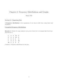
4 Each case falls into only one interval Every case is assigned somewhereCOMPUTE age10 = age .RECODE age10(18 thru 19=1) (20 thru 29=2) (30 thru 39=3) (40 thru 49=4) (50 thru 59=5) (60 thru 69=6) (70 thru 79=7) (80 thru 89=8) (ELSE=SYSMIS) . variable LABELS age10 AGE IN DECADES' .VALUE LABELS age101 '18-19' 2 '20-29' 3 '30-39' 4 '40-49' 5 '50-59' 6 '60-69' 7 '70-79' 8 '80-89' .FREQUENCIES Variables = age age10 .AGE in the 2008 GSS Respondent s AGEis coded in years, 72categories from 18 to 89 (and 10 cases with missing data, coded = 99).Let s use these SPSS commands to collapse AGEinto eight decades, by creating a new variable called AGE10:AGE Age of RespondentFrequencyPercentValid PercentCumulative ** + ** 66 rows deleted hereAGE10 Age in DecadesWhich decade(s) has the most cases?

5 _____Which has the largest percentage? _____FrequencyPercentValid PercentCumulative Type of Grouped DataOrdered frequency distributions may be tabled withoutcollapsed any categories. Although each score doesn t involve a range from lower to upper limits, I also refer to such tabular displays as grouped data because each category represents numerous respondents:NEWSHOW OFTEN DOES R READ NEWSPAPERF requencyValid %1 FEW TIMES A ONCE A LESS THAN ONCE the poor GSS practice of assigning higher numbers to lower-level activity! You should recode to reverse their DistributionsCumulative frequency :for a given score or outcome of a variable , the total number of cases in the distribution at or below that valueCumulation makes sense only for orderable discrete and continuous should you never make a cumulative frequency distribution for a nonorderable discrete variable , such as race or state of residence?

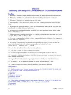
6 Both cumulative frequency distributionsand cumulative percentage distributionsare created by adding the counts or the %s in the lower-valued categoriesFor an example, see the Cumulative Percent in the preceding AGE10 tableWhat % of 2008 GSS are < 60 years old? _____Graphing frequency DistributionsA Graphor Diagramvisually summarizes the numbers in a frequency distribution or other basic types of graphs:BAR CHARTfor nonordered discrete variablesHISTOGRAMfor ordered discrete variablesPOLYGONfor continuous variablesOn the following slides, how do bar charts and histograms differ in the spaces between their bars? Why?How does a histogram differ from a polygon?

7 NEW ENGLANDMIDDLE ATLANTICE. NOR. CENTRALW. NOR. CENTRALSOUTH ATLANTICE. SOU. CENTRALW. SOU. CENTRALMOUNTAINPACIFICREGION OF INTERVIEW0100200300400500 CountBar Chart of REGIONH istogram of AGE100123456789 AGE IN DECADES0100200300400 CountPolygon of AGE1018-1920-2930-3940-4950-5960-6970-79 80-89 AGE IN DECADES0100200300400 CountVariations on Basic GraphsTwo histograms: Age pyramids by sexTwo polygons: Approval over time12 bar charts: Opinion by nationROUNDING RULES from Box Round digits 1 to 4 down by leaving the digit to the left unchanged. 2. Round digits 6 to 9 up by increasing the digit to the left by 1. 3. Numbers ending in 5 are rounded alternately; the first number ending in 5 is rounded down, the second is rounded up, the third is rounded down, and so forth.

8 Round past the original measurement interval. Examples:Unit of MeasurementYears (tenths) Rounded