Transcription of CHAPTER 2 Estimating Probabilities
1 CHAPTER 2 Estimating ProbabilitiesMachine LearningCopyrightc 2017. Tom M. Mitchell. All rights reserved.*DRAFT OF January 26, 2018**PLEASE DO NOT DISTRIBUTE WITHOUT AUTHOR SPERMISSION*This is a rough draft CHAPTER intended for inclusion in the upcoming secondedition of the textbookMachine Learning, Mitchell, McGraw are welcome to use this for educational purposes, but do not duplicateor repost it on the internet. For online copies of this and other materialsrelated to this book, visit the web site send suggestions for improvements, or suggested exercises, machine learning methods depend on probabilistic approaches.
2 Thereason is simple: when we are interested in learning some target functionf:X Y, we can more generally learn the probabilistic functionP(Y|X).By using a probabilistic approach, we can design algorithms that learn func-tions with uncertain outcomes ( , predicting tomorrow s stock price) andthat incorporate prior knowledge to guide learning ( , a bias that tomor-row s stock price is likely to be similar to today s price). This CHAPTER de-scribes joint probability distributions over many variables, and shows howthey can be used to calculate a targetP(Y|X). It also considers the problemof learning, or Estimating , probability distributions from training data, pre-senting the two most common approaches: maximum likelihood estimationand maximum a posteriori Joint probability DistributionsThe key to building probabilistic models is to define a set of random variables,and to consider the joint probability distribution over them.
3 For example, Table1 defines a joint probability distribution over three random variables: a person s1 Copyrightc 2016, Tom M. HoursWorked Wealthprobabilityfemale< < < < 1:A Joint probability table defines a joint probability distri-bution over three random variables: Gender, HoursWorked, and , the number of HoursWorked each week, and their Wealth. In general,defining a joint probability distribution over a set of discrete-valued variables in-volves three simple steps:1. Define the random variables, and the set of values each variable can takeon. For example, in Table 1 the variableGendercan take on the valuemaleorfemale, the variableHoursWorkedcan take on the value < or , andWealthcan take on Create a table containing one row for each possible joint assignment of val-ues to the variables.
4 For example, Table 1 has 8 rows, corresponding to the 8possible ways of jointly assigning values to three boolean-valued generally, if we havenboolean valued variables, there will be 2nrowsin the Define a probability for each possible joint assignment of values to the vari-ables. Because the rows cover every possible joint assignment of values,their Probabilities must sum to joint probability distribution is central to probabilistic inference, becauseonce we know the joint distribution we can answer every possible probabilisticquestion that can be asked about these variables. We can calculate conditional orjoint Probabilities overanysubset of the variables, given their joint is accomplished by operating on the Probabilities for the relevant rows in thetable.
5 For example, we can calculate: The probability that any single variable will take on any specific value. Forexample, we can calculate that the probabilityP(Gender=male) = the joint distribution in Table 1, by summing the four rows for whichGender = male. Similarly, we can calculate the probabilityP(Wealth=rich) = by adding together the Probabilities for the four rows cover-ing the cases for whichWealth= 2016, Tom M. The probability that any subset of the variables will take on a particular jointassignment. For example, we can calculate that the probabilityP(Wealth=rich Gender=female) = , by summing the two table rows that satisfy thisjoint assignment.
6 Any conditional probability defined over subsets of the variables. Recallthe definition of conditional probabilityP(Y|X) =P(X Y)/P(X). We cancalculate both the numerator and denominator in this definition by sum-ming appropriate rows, to obtain the conditional probability . For example,according to Table 1,P(Wealth=rich|Gender=female) = summarize, if we know the joint probability distribution over an arbi-trary set of random variables{ }, then we can calculate the conditionaland joint probability distributions for arbitrary subsets of these variables ( ,P(Xn| 1)). In theory, we can in this way solve any classification, re-gression, or other function approximation problem defined over these variables,and furthermore produce probabilistic rather than deterministic predictions forany given input to the target example, if we wish to learn topredict which people are rich or poor based on their gender and hours worked,we can use the above approach to simply calculate the probability distributionP(Wealth|Gender, HoursWorked).
7 Learning the Joint DistributionHow can we learn joint distributions from observed training data? In the exampleof Table 1 it will be easy if we begin with a large database containing, say, descrip-tions of a million people in terms of their values for our three variables. Given alarge data set such as this, one can easily estimate a probability for each row in thetable by calculating the fraction of database entries (people) that satisfy the jointassignment specified for that row. If thousands of database entries fall into eachrow, we will obtain highly reliable probability estimates using this other cases, however, it can be difficult to learn the joint distribution due tothe very large amount of training data required.
8 To see the point, consider how ourlearning problem would change if we were to add additional variables to describea total of 100 boolean features for each person in Table 1 ( , we could add dothey have a college degree? , are they healthy? ). Given 100 boolean features,the number of rows in the table would now expand to 2100, which is greater than1030. Unfortunately, even if our database describes every single person on earthwe would not have enough data to obtain reliable probability estimates for mostrows. There are only approximately 1010people on earth, which means that formost of the 1030rows in our table, we would have zero training examples!
9 This1Of course if our random variables have continuous values instead of discrete, we would needan infinitely large table. In such cases we represent the joint distribution by a function instead of atable, but the principles for using the joint distribution remain 2016, Tom M. a significant problem given that real-world machine learning applications oftenuse many more than 100 features to describe each example for example, manylearning algorithms for text analysis use millions of features to describe text in agiven successfully address the issue of learning Probabilities from available train-ing data, we must (1) be smart about how we estimate probability parameters fromavailable data, and (2)
10 Be smart about how we represent joint probability Estimating ProbabilitiesLet us begin our discussion of how to estimate Probabilities with a simple exam-ple, and explore two intuitive algorithms. It will turn out that these two intuitivealgorithms illustrate the two primary approaches used in nearly all probabilisticmachine learning this simple example you have a coin, represented by the random variableX. If you flip this coin, it may turn up heads (indicated byX=1) or tails (X=0).The learning task is to estimate the probability that it will turn up heads; that is, toestimateP(X=1). We will use to refer to the true (but unknown) probability ofheads ( ,P(X=1) = ), and use to refer to our learned estimate of this true.