Transcription of CHAPTER 2: Limits and Continuity - kkuniyuk.com
1 CHAPTER 2: Limits and Continuity : An Introduction to Limits : Properties of Limits : Limits and Infinity I: Horizontal Asymptotes (HAs) : Limits and Infinity II: Vertical Asymptotes (VAs) : The Indeterminate Forms 0/0 and / : The Squeeze (Sandwich) Theorem : Precise Definitions of Limits : Continuity The conventional approach to calculus is founded on Limits . In this CHAPTER , we will develop the concept of a limit by example. Properties of Limits will be established along the way. We will use Limits to analyze asymptotic behaviors of functions and their graphs. Limits will be formally defined near the end of the CHAPTER . Continuity of a function (at a point and on an interval) will be defined using Limits . (Section : An Introduction to Limits ) : AN INTRODUCTION TO Limits LEARNING OBJECTIVES Understand the concept of (and notation for) a limit of a rational function at a point in its domain, and understand that Limits are local.
2 Evaluate such Limits . Distinguish between one-sided (left-hand and right-hand) Limits and two-sided Limits and what it means for such Limits to exist. Use numerical / tabular methods to guess at limit values. Distinguish between limit values and function values at a point. Understand the use of neighborhoods and punctured neighborhoods in the evaluation of one-sided and two-sided Limits . Evaluate some Limits involving piecewise-defined functions. PART A: THE LIMIT OF A FUNCTION AT A POINT Our study of calculus begins with an understanding of the expression limx afx(), where a is a real number (in short, a ) and f is a function. This is read as: the limit of fx() as x approaches a. WARNING 1: means approaches. Avoid using this symbol outside the context of Limits . limx a is called a limit operator. Here, it is applied to the function f.
3 Limx afx() is the real number that fx() approaches as x approaches a, if such a number exists. If fx() does, indeed, approach a real number, we denote that number by L (for limit value). We say the limit exists, and we write: limx afx()=L, or fx() L as x a. These statements will be rigorously defined in Section (Section : An Introduction to Limits ) When we evaluate limx afx(), we do one of the following: We find the limit value L (in simplified form). We write: limx afx()=L. We say the limit is (infinity) or (negative infinity). We write: limx afx()= , or limx afx()= . We say the limit does not exist ( DNE ) in some other way. We write: limx afx() DNE. (The DNE notation is used by Swokowski but few other authors.) If we say the limit is or , the limit is still nonexistent. Think of and as special cases of DNE that we do write when appropriate; they indicate why the limit does not exist.
4 Limx afx() exists does not exist The limit is a real number, L. DNE limx afx() is called a limit at a point, because x=a corresponds to a point on the real number line. Sometimes, this is related to a point on the graph of f . Example 1 (Evaluating the Limit of a Polynomial Function at a Point) Let fx()=3x2+x 1. Evaluate limx 1fx(). Solution f is a polynomial function with implied domain Domf()= . We substitute ( plug in ) x=1 and evaluate f1(). WARNING 2: Sometimes, the limit value limx afx() does not equal the function value fa(). (See Part C.) (Section : An Introduction to Limits ) limx 1fx()=limx 13x2+x 1() WARNING 3: Use grouping symbols when taking the limit of an expression consisting of more than one term. =31()2+1() 1 WARNING 4: Do not omit the limit operator limx 1 until this substitution phase.
5 WARNING 5: When performing substitutions, be prepared to use grouping symbols. Omit them only if you are sure they are unnecessary. =3 We can write: limx 1fx()=3, or fx() 3 as x 1. Be prepared to work with function and variable names other than f and x. For example, if gt()=3t2+t 1, then limt 1gt()=3, also. The graph of y=fx() is below. Imagine that the arrows in the figure represent two lovers running towards each other along the parabola. What is the y-coordinate of the point they are approaching as they approach x=1? It is 3, the limit value. TIP 1: Remember that y-coordinates of points along the graph correspond to function values. (Section : An Introduction to Limits ) Example 2 (Evaluating the Limit of a rational Function at a Point) Let fx()=2x+1x 2. Evaluate limx 3fx(). Solution f is a rational function with implied domain Domf()=x x 2{}.
6 We observe that 3 is in the domain of f in short, 3 Domf()(), so we substitute ( plug in ) x=3 and evaluate f3(). limx 3fx()=limx 32x+1x 2=23()+13() 2=7 The graph of y=fx() is below. Note: As is often the case, you might not know how to draw the graph until later. Asymptotes. The dashed lines are asymptotes, which are lines that a graph approaches - in a long-run sense (see the horizontal asymptote, or HA, at y=2), or - in an explosive sense (see the vertical asymptote, or VA, at x=2). HA s and VA s will be defined using Limits in Sections and , respectively. (Section : An Introduction to Limits ) Limits are Local. What if the lover on the left is running along the left branch of the graph? In fact, we ignore the left branch, because of the following key principle of Limits . Limits [at a Point] are Local When analyzing limx afx(), we only consider the behavior of f in the immediate vicinity of x=a.
7 In fact, we may exclude consideration of x=a itself, as we will see in Part C. In the graph, we only care what happens immediately around x=3. Section will feature a rigorous approach. Example 3 (Evaluating the Limit of a Constant Function at a Point) limx 2=2. (Observe that substituting x= technically works here, since there is no x in 2, anyway.) A constant approaches itself. We can write 2 2 ( 2 approaches 2 ) as x . When we think of a sequence of numbers approaching 2, we may think of distinct numbers such as , , , .. However, the constant sequence 2, 2, 2, .. is also said to approach 2. All constant functions are also polynomial functions, and all polynomial functions are also rational functions. The following theorem applies to all three Examples thus far. Basic Limit Theorem for rational Functions If f is a rational function, and a Domf(), then limx afx()=fa().
8 To evaluate the limit, substitute ( plug in ) x=a, and evaluate fa(). We will justify this theorem in Section (Section : An Introduction to Limits ) PART B: ONE- AND TWO-SIDED Limits ; EXISTENCE OF Limits limx a is a two-sided limit operator in limx afx(), because we must consider the behavior of f as x approaches a from both the left and the right. limx a is a one-sided left-hand limit operator. limx a fx() is read as: the limit of fx() as x approaches a from the left. limx a+ is a one-sided right-hand limit operator. limx a+fx() is read as: the limit of fx() as x approaches a from the right. Example 4 (Using a Numerical / Tabular Approach to Guess a Left-Hand Limit Value) Guess the value of limx 3 x+3() using a table of function values. Solution Let fx()=x+3. limx 3 fx() is the real number, if any, that fx() approaches as x approaches 3 from lesser (or lower) numbers.
9 That is, we approach x=3 from the left along the real number line. We select an increasing sequence of real numbers (x values) approaching 3 such that all the numbers are close to (but less than) 3. We evaluate the function at those numbers, and we guess the limit value, if any, the function values are approaching. For example: x 3 fx()=x+3 6 (?) We guess: limx 3 x+3()=6. WARNING 6: Do not confuse superscripts with signs of numbers. Be careful about associating the superscript with negative numbers. Here, we consider positive numbers that are close to 3. If we were taking a limit as x approached 0, then we would associate the superscript with negative numbers and the + superscript with positive numbers. (Section : An Introduction to Limits ) The graph of y=fx() is below. We only consider the behavior of f immediately to the left of x=3.
10 WARNING 7: The numerical / tabular approach is unreliable, and it is typically unacceptable as a method for evaluating Limits on exams. (See Part D, Example 11 to witness a failure of this method.) However, it may help us guess at limit values, and it strengthens our understanding of Limits . Example 5 (Using a Numerical / Tabular Approach to Guess a Right-Hand Limit Value) Guess the value of limx 3+x+3() using a table of function values. Solution Let fx()=x+3. limx 3+fx() is the real number, if any, that fx() approaches as x approaches 3 from greater (or higher) numbers. That is, we approach x=3 from the right along the real number line. We select a decreasing sequence of real numbers (x values) approaching 3 such that all the numbers are close to (but greater than) 3. We evaluate the function at those numbers, and we guess the limit value, if any, the function values are approaching.