Transcription of Chapter 3: Methods for Generating Random Variables
1 Chapter 3: Methods for GeneratingRandom VariablesLecturer: Zhao JianhuaDepartment of StatisticsYunnan University of Finance and IntroductionRandom Generators of Common Probability Distributions in The Inverse Transform Inverse Transform Method, Continuous Inverse Transform Method, Discrete The Acceptance-Rejection MethodThe Acceptance-Rejection Transformation Sums and Multivariate Multivariate Normal Mixtures of Multivariate Wishart Uniform Dist. on thed-SphereIntroduction One of the fundamental tools required in computational statis-tics is the ability to simulate Random Variables ( ) from spec-ified probability (prob.) distributions (dist.). A suitable generator of uniform pseudo Random numbers is es-sential. Methods for Generating from other prob. dist. alldepend on the uniform Random number : Generating Uniform Random (n) #generate a vector of size n in [0,1]runif(n,a,b) #generate n Uniform(a, b) numbersmatrix(runif(n*m),n,m) #generate n by m matrixThesamplefunction can be used to sample from a finite population,with or without (Sampling from a finite population)> #toss some coins> sample (0:1, size = 10, replace = TRUE)> #choose some lottery numbers> sample (1:100 , size = 6, replace = FALSE)> #permuation of letters a-z> sample(letters)> #sample from a multinomial dist.
2 > x=sample (1:3, size =100, replace=TRUE ,prob=c(.2 ,.3 ,.5))> table(x)x1 2 317 35 48 Random Generators of Common Prob. Dist. in RThe prob. mass function (pmf) or density (pdf), cumulative dist. function(cdf), quantile function, and Random generator of many commonly usedprob. dist. are available. For example:dbinom(x,size ,prob ,log = FALSE ); rbinom(n,size ,prob)pbinom(q,size ,prob , , )qbinom(p,size ,prob , , )Table: Selected Univariate Prob. Functions Available in RDistributioncdfGeneratorParametersbetap betarbetashape1, shape2binomialpbinomrbinomsize, probchi-squaredpchisqrchisqdfexponential pexprexprateFpfrfdf1, df2gammapgamma rgamma shape, rate or scalegeometricpgeomrgeomproblognormalpln ormrlnormmeanlog, sdlognegative binomial pnbinom rnbinomsize, probnormalpnormrnormmean, sdPoissonppoisrpoislambdaStudents tptrtdfuniformpunifrunifmin, maxThe Inverse Transform MethodTheorem: IfXis a continuous with CDFFX(x), thenU=FX(X) U(0,1).
3 Proof:FX(x) =P(X x) =P(FX(X) FX(x)) =P(U FX(x)). Second=is becauseFX(x)is an increasing function. Bythe definition of uniform CDF, we haveU U(0,1).Define: the inverse transformationF 1X(u) =inf{x:FX(x) =u},0< u < U(0,1), then for allx R,P(F 1X(U) x) =P(inf{t:FX(t) =U} x)=P(U FX(x)) =FU(FX(x)) =FX(x),and thereforeF 1X(U)has the same dist. generate a Random observationX, the inverse functionF 1X(u) a randomufromU(0,1). 1X(u).The method easy to apply, provided thatF 1 Xis easy to Transform Method, Continuous CaseExample (Inverse transform method, continuous case)Simulate a Random sample from the dist. with densityfX(x) = 3x2,0< x < (x) =x3for0< x <1, andF 1X(u) =u1/3, thenn <- 1000 ; u <- runif(n) ; x <- u^(1/3)hist(x, prob = TRUE) #density histogram of sampley <- seq (0 ,1.)
4 01); lines(y,3*y^2) #density curve f(x)f(x)= histogramwith theoretical densityf(x) = note Figure , the title includes a math expression, obtained byhist(x, prob = TRUE , main = expression(f(x)==3*x^2)).Alternately,mai n = bquote(f(x)==3*x^2))produces the sametitle. Math annotation is covered in the help topic see the help topics (Exponential dist.)Generate a Random sample from the exponential Exp( ), forx >0, the cdf ofXisFX(x) = 1 e x, thenF 1(u) = 1 log(1 u). Note thatUand1 Uhave the samedist. and it is simpler to setx= 1 log(u). To generate a randomsample of sizenwith parameterlambda:-log(runif(n)) / lambdaA generatorrexpis available in Transform Method, Discrete CaseIf X is a discrete and < xi 1< xi< xi+1< are the points of discontinuity ofFX(x).Define:F 1X(u) =inf{x:FX(x) u}then the inverse transformation isF 1X(u) =xi, whereFX(xi 1)<u FX(xi).
5 For each Random variate a randomufromU(0,1). (xi 1)< u F(xi).The solution ofFX(xi 1)< u FX(xi)may be difficult for (Two point distribution)Generate a Random sample of Bernoulli(p= ) this example,FX(0) =fX(0) = 1 pandFX(1) = ,F 1X(u) = 1,ifu > (u) = 0ifu ,n <- 1000 ; p< ; u <- runif(n)x <- (u > ) #(u > ) is a logical vector> mean(x);var(x)[1] mean and variance should be approximatelyp= (1 p) = note ( Random binomial) function withsize=1generates aBernoulli sample. Another method is to sample from the vector(0,1)with prob.(1 p,p).rbinom(n, size = 1, prob = p)sample(c(0,1),size=n,replace=TRUE ,prob = c(.6 ,.4))Example (Geometric distribution)Generate a Random geometric sample with parameterp= pmf isf(x) =pqx,x= 0,1,2, , whereq= 1 p. At thepoints of discontinuityx= 0,1,2, , cdf isF(x) = 1 qx+1.
6 Foreach sample element, we generate a Random uniformuand solve1 qx< u 1 qx,which simplifies tox <log (1 u)/log (q) x+ 1. Thusx+ 1 =dlog (1 u)/log (q)e, wheredtedenotes ceiling <- 1000p <- <- runif(n)k <- ceiling(log(1-u) / log(1-p)) - 1 Uand1 Uhave the same dist. and the prob. thatlog(1 u)/log(1 p)equals an integer is zero, and thus the last step isk <- floor(log(u) / log(1-p))Poisson distributionThe basic method to generate a Poisson( ) variate is to generateand store the cdf via the recursive formulaf(x+ 1) = f(x)x+ 1;F(x+ 1) =F(x) +f(x+ 1).For each Poisson variate , a Random uniformuis generated, and thecdf vector is searched for the solution toF(x 1)< u F(x).Note:R functionrpoisgenerates Random Poisson (Logarithmic distribution)Simulate a Logarithmic( ) Random samplef(x) =P(X=x) =a xx,x= 1,2, ( )where0< <1anda= ( log(1 )) recursive formula forf(x)isf(x+ 1) = xx+ 1f(x),x= 1,2, ( )Generate Random samples from Logarithmic( ) <- 1000 ; theta <- ; x <- rlogarithmic(n, theta)#compute density of logarithmic(theta) for comparisonk<-sort(unique(x)); p=-1/log(1-theta)*theta^k/kse<-sqrt(p*(1 -p)/n) #standard errorSample relative frequencies (line 1) match theoretical dist.
7 (line 2)of Logarithmic( ) dist. within two standard errors.> round(rbind(table(x)/n, p, se),3)1 2 3 4 5 6 Initially choose a lengthNfor the cdf vector, and computeF(x),x= 1,2, ,N. If necessary,Nwill be <- function(n, theta) {#returns a Random logarithmic(theta) sample size nu <- runif(n)#set the initial length of cdf vectorN <- ceiling (-16 / log10(theta))k <- 1:N; a <- -1/log(1-theta)fk <- a*theta^k/kFk <- cumsum(fk); x <- integer(n)for (i in 1:n) {x[i] <- (sum(u[i] > Fk)) #F^{-1}(u)-1while (x[i] == N) {#if x==N we need to extend the cdf#very unlikely because N is largef <- a*theta^(N+1)/Nfk <- c(fk, f)Fk <- c(Fk, Fk[N] + fk[N+1])N <- N + 1x[i] <- (sum(u[i] > Fk))}}x + 1 }The Acceptance-Rejection MethodSuppose thatXandYare with density or pmffandgre-spectively, and there exists a constantcsuch thatf(t)g(t) cfor alltsuch thatf(t)> the acceptance-rejection method can beapplied to generate the acceptance-rejection a densitygsatisfyingf(t)/g(t) c,for alltsuch thatf(t)> a randomyfrom the dist.
8 With a randomufrom theU(0,1) < f(y)/(cg(y))acceptyand deliverx=y; otherwiserejectyand repeat step that in step 4,P(accept|Y) =P(U <f(Y)cg(Y)|Y) =f(Y)cg(Y).The total prob. of acceptance for any iteration is yP(accept|y)P(Y=y) = yf(y)cg(y)g(y) = the discrete case, for eachksuch thatf(k)>0,P(Y=k|A) =P(A|k)g(k)P(A)=(f(k)cg(k))g(k)1/c=f(k)I n the continuous case, we need to proveP(Y y|U f(Y)cg(Y)) =FX(y).In factP(Y y|U f(Y)cg(Y))=P(U f(Y)cg(Y),Y y)1/c= y P(U f(Y)cg(Y)|Y= y)1/cg( )d =c y f( )cg( )g( )d =FX(y)Example (Acceptance-rejection method), Beta( = 2, = 2) Beta(2,2) density isf(x) = 6x(1 x),0< x <1. Letg(x)be theU(0,1)density. Thenf(x)/g(x) 6for all0< x <1,soc= randomxfromg(x)is accepted iff(x)/cg(x) =x(1 x)> ,cn= 6000 iterations will be required for sample size <- 1000; k <- 0 #counter for acceptedy <- numeric(n); j <- 0 #iterationswhile (k < n) {u <- runif (1); j<-j+1;x <- runif (1) # Random variate from gif (x * (1-x) > u) { k<-k+1; y[k] <- x }} #we accept x>j[1] 5873 This simulation required 5873 iterations (11746 Random numbers).
9 #compare empirical and theoretical percentilesp<-seq (.1 ,.9 ,.1); Qhat <-quantile(y,p) #quantiles of sampleQ <- qbeta(p, 2, 2) #theoretical quantilesse <- sqrt(p * (1-p) / (n * dbeta(Q, 2, 2))) #see Ch. 1 Sample percentiles (line 1) approximately match the Beta(2,2) per-centiles computed byqbeta(line 2).> round(rbind(Qhat , Q, se), 3)10% 20% 30% 40% 50% 60% 70% 80% 90%Qhat 10000replicates produces more precise estimates.> round(rbind(Qhat , Q, se), 3)10% 20% 30% 40% 50% 60% 70% 80% 90%Qhat numbers of replicates are required for estimation of percentileswhere the density is close to Example for a more efficient beta generator based on theratio of gammas MethodsMany types of transformations other than the prob.
10 Inverse trans-formation can be applied to simulate N(0,1),thenV=Z2 2(1). 2(m)andV 2(n)are independent, thenF=V/mU/m F(m,n). N(0,1)andV 2(n)are independent, thenT=Z V/n t(n) ,V U(0,1)are independent, thenZ1= 2 logUcos (2 V)Z2= 2 logVsin (2 U)are independent standard Gamma(r, )andV Gamma(s, )are independent,thenX=U/(U+V)has the Beta(r,s) ,V U(0,1)are independent, thenX=b1+log (V)log (1 (1 )U)chas the Logarithmic() dist., wherebxcdenotes the integer (Beta distribution)IfU Gamma(r, )andV Gamma(s, )are independent, thenX=U/(U+V)has the Beta(r,s) Gamma(a,1). Gamma(b,1). (u+v).Beta(3,2) samplen <- 1000; a <- 3; b <- 2;u <- rgamma(n, shape=a, rate =1);v <- rgamma(n, shape=b, rate =1);x <- u/(u + v)q <- qbeta(ppoints(n), a, b)qqplot(q, x, cex = , xlab="Beta(3, 2)", ylab="Sample")abline(0, 1) #line x = q added for sample data can be compared with the Beta(3, 2) dist.