Transcription of Chapter 3: Methods for Generating Random Variables
1 Chapter 3: Methods for GeneratingRandom VariablesLecturer: Zhao JianhuaDepartment of StatisticsYunnan University of Finance and IntroductionRandom Generators of Common probability Distributions in The Inverse Transform Inverse Transform Method, continuous Inverse Transform Method, Discrete The Acceptance-Rejection MethodThe Acceptance-Rejection Transformation Sums and Multivariate Multivariate Normal Mixtures of Multivariate Wishart Uniform Dist. on thed-SphereIntroduction One of the fundamental tools required in computational statis-tics is the ability to simulate Random Variables ( ) from spec-ified probability (prob.) distributions (dist.). A suitable generator of uniform pseudo Random numbers is es-sential.
2 Methods for Generating from other prob. dist. alldepend on the uniform Random number : Generating Uniform Random (n) #generate a vector of size n in [0,1]runif(n,a,b) #generate n Uniform(a, b) numbersmatrix(runif(n*m),n,m) #generate n by m matrixThesamplefunction can be used to sample from a finite population,with or without (Sampling from a finite population)> #toss some coins> sample (0:1, size = 10, replace = TRUE)> #choose some lottery numbers> sample (1:100 , size = 6, replace = FALSE)> #permuation of letters a-z> sample(letters)> #sample from a multinomial dist.> x=sample (1:3, size =100, replace=TRUE ,prob=c(.2 ,.3 ,.5))> table(x)x1 2 317 35 48 Random Generators of Common Prob. Dist. in RThe prob. mass function (pmf) or density (pdf), cumulative dist.
3 Function(cdf), quantile function, and Random generator of many commonly usedprob. dist. are available. For example:dbinom(x,size ,prob ,log = FALSE ); rbinom(n,size ,prob)pbinom(q,size ,prob , , )qbinom(p,size ,prob , , )Table: Selected Univariate Prob. Functions Available in RDistributioncdfGeneratorParametersbetap betarbetashape1, shape2binomialpbinomrbinomsize, probchi-squaredpchisqrchisqdfexponential pexprexprateFpfrfdf1, df2gammapgamma rgamma shape, rate or scalegeometricpgeomrgeomproblognormalpln ormrlnormmeanlog, sdlognegative binomial pnbinom rnbinomsize, probnormalpnormrnormmean, sdPoissonppoisrpoislambdaStudents tptrtdfuniformpunifrunifmin, maxThe Inverse Transform MethodTheorem: IfXis a continuous with CDFFX(x), thenU=FX(X) U(0,1).
4 Proof:FX(x) =P(X x) =P(FX(X) FX(x)) =P(U FX(x)). Second=is becauseFX(x)is an increasing function. Bythe definition of uniform CDF, we haveU U(0,1).Define: the inverse transformationF 1X(u) =inf{x:FX(x) =u},0< u < U(0,1), then for allx R,P(F 1X(U) x) =P(inf{t:FX(t) =U} x)=P(U FX(x)) =FU(FX(x)) =FX(x),and thereforeF 1X(U)has the same dist. generate a Random observationX, the inverse functionF 1X(u) a randomufromU(0,1). 1X(u).The method easy to apply, provided thatF 1 Xis easy to Transform Method, continuous CaseExample (Inverse transform method, continuous case)Simulate a Random sample from the dist. with densityfX(x) = 3x2,0< x < (x) =x3for0< x <1, andF 1X(u) =u1/3, thenn <- 1000 ; u <- runif(n) ; x <- u^(1/3)hist(x, prob = TRUE) #density histogram of sampley <- seq (0 ,1.)
5 01); lines(y,3*y^2) #density curve f(x)f(x)= histogramwith theoretical densityf(x) = note Figure , the title includes a math expression, obtained byhist(x, prob = TRUE , main = expression(f(x)==3*x^2)).Alternately,mai n = bquote(f(x)==3*x^2))produces the sametitle. Math annotation is covered in the help topic see the help topics (Exponential dist.)Generate a Random sample from the exponential Exp( ), forx >0, the cdf ofXisFX(x) = 1 e x, thenF 1(u) = 1 log(1 u). Note thatUand1 Uhave the samedist. and it is simpler to setx= 1 log(u). To generate a randomsample of sizenwith parameterlambda:-log(runif(n)) / lambdaA generatorrexpis available in Transform Method, Discrete CaseIf X is a discrete and < xi 1< xi< xi+1< are the points of discontinuity ofFX(x).
6 Define:F 1X(u) =inf{x:FX(x) u}then the inverse transformation isF 1X(u) =xi, whereFX(xi 1)<u FX(xi).For each Random variate a randomufromU(0,1). (xi 1)< u F(xi).The solution ofFX(xi 1)< u FX(xi)may be difficult for (Two point distribution)Generate a Random sample of Bernoulli(p= ) this example,FX(0) =fX(0) = 1 pandFX(1) = ,F 1X(u) = 1,ifu > (u) = 0ifu ,n <- 1000 ; p< ; u <- runif(n)x <- (u > ) #(u > ) is a logical vector> mean(x);var(x)[1] mean and variance should be approximatelyp= (1 p) = note ( Random binomial) function withsize=1generates aBernoulli sample. Another method is to sample from the vector(0,1)with prob.(1 p,p).rbinom(n, size = 1, prob = p)sample(c(0,1),size=n,replace=TRUE ,prob = c(.6 ,.4))Example (Geometric distribution)Generate a Random geometric sample with parameterp= pmf isf(x) =pqx,x= 0,1,2, , whereq= 1 p.
7 At thepoints of discontinuityx= 0,1,2, , cdf isF(x) = 1 qx+1. Foreach sample element, we generate a Random uniformuand solve1 qx< u 1 qx,which simplifies tox <log (1 u)/log (q) x+ 1. Thusx+ 1 =dlog (1 u)/log (q)e, wheredtedenotes ceiling <- 1000p <- <- runif(n)k <- ceiling(log(1-u) / log(1-p)) - 1 Uand1 Uhave the same dist. and the prob. thatlog(1 u)/log(1 p)equals an integer is zero, and thus the last step isk <- floor(log(u) / log(1-p))Poisson distributionThe basic method to generate a Poisson( ) variate is to generateand store the cdf via the recursive formulaf(x+ 1) = f(x)x+ 1;F(x+ 1) =F(x) +f(x+ 1).For each Poisson variate, a Random uniformuis generated, and thecdf vector is searched for the solution toF(x 1)< u F(x).
8 Note:R functionrpoisgenerates Random Poisson (Logarithmic distribution)Simulate a Logarithmic( ) Random samplef(x) =P(X=x) =a xx,x= 1,2, ( )where0< <1anda= ( log(1 )) recursive formula forf(x)isf(x+ 1) = xx+ 1f(x),x= 1,2, ( )Generate Random samples from Logarithmic( ) <- 1000 ; theta <- ; x <- rlogarithmic(n, theta)#compute density of logarithmic(theta) for comparisonk<-sort(unique(x)); p=-1/log(1-theta)*theta^k/kse<-sqrt(p*(1-p)/n) #standard errorSample relative frequencies (line 1) match theoretical dist. (line 2)of Logarithmic( ) dist. within two standard errors.> round(rbind(table(x)/n, p, se),3)1 2 3 4 5 6 Initially choose a lengthNfor the cdf vector, and computeF(x),x= 1,2, ,N.
9 If necessary,Nwill be <- function(n, theta) {#returns a Random logarithmic(theta) sample size nu <- runif(n)#set the initial length of cdf vectorN <- ceiling (-16 / log10(theta))k <- 1:N; a <- -1/log(1-theta)fk <- a*theta^k/kFk <- cumsum(fk); x <- integer(n)for (i in 1:n) {x[i] <- (sum(u[i] > Fk)) #F^{-1}(u)-1while (x[i] == N) {#if x==N we need to extend the cdf#very unlikely because N is largef <- a*theta^(N+1)/Nfk <- c(fk, f)Fk <- c(Fk, Fk[N] + fk[N+1])N <- N + 1x[i] <- (sum(u[i] > Fk))}}x + 1 }The Acceptance-Rejection MethodSuppose thatXandYare with density or pmffandgre-spectively, and there exists a constantcsuch thatf(t)g(t) cfor alltsuch thatf(t)> the acceptance-rejection method can beapplied to generate the acceptance-rejection a densitygsatisfyingf(t)/g(t) c,for alltsuch thatf(t)> a randomyfrom the dist.
10 With a randomufrom theU(0,1) < f(y)/(cg(y))acceptyand deliverx=y; otherwiserejectyand repeat step that in step 4,P(accept|Y) =P(U <f(Y)cg(Y)|Y) =f(Y)cg(Y).The total prob. of acceptance for any iteration is yP(accept|y)P(Y=y) = yf(y)cg(y)g(y) = the discrete case, for eachksuch thatf(k)>0,P(Y=k|A) =P(A|k)g(k)P(A)=(f(k)cg(k))g(k)1/c=f(k)I n the continuous case, we need to proveP(Y y|U f(Y)cg(Y)) =FX(y).In factP(Y y|U f(Y)cg(Y))=P(U f(Y)cg(Y),Y y)1/c= y P(U f(Y)cg(Y)|Y= y)1/cg( )d =c y f( )cg( )g( )d =FX(y)Example (Acceptance-rejection method), Beta( = 2, = 2) Beta(2,2) density isf(x) = 6x(1 x),0< x <1. Letg(x)be theU(0,1)density. Thenf(x)/g(x) 6for all0< x <1,soc= randomxfromg(x)is accepted iff(x)/cg(x) =x(1 x)> ,cn= 6000 iterations will be required for sample size <- 1000; k <- 0 #counter for acceptedy <- numeric(n); j <- 0 #iterationswhile (k < n) {u <- runif (1); j<-j+1;x <- runif (1) # Random variate from gif (x * (1-x) > u) { k<-k+1; y[k] <- x }} #we accept x>j[1] 5873 This simulation required 5873 iterations (11746 Random numbers).