Chapter 3. Multivariate Distributions.

1 3-1 Chapter 3. Multivariate of the most interesting problems in statistics involve looking at more than a single measurementat a time, at relationships among measurements and comparisons between them. In order to permit us toaddress such problems, indeed to even formulate them properly, we will need to enlarge our mathematicalstructure to includemultivariate distributions,the probability distributions of pairs of random variables,triplets of random variables, and so forth. We will begin with the simplest such situation, that of pairs ofrandom variables orbivariate distributions,where we will already encounter most of the key Discrete Bivariate two random variables defined on the same sample spaceS; that is, defined in referenceto the same experiment, so that it is both meaningful and potentially interesting to consider how they mayinteract or affect one another, we will define theirbivariate probability functionbyp(x, y) =P(X=xandY=y).

2 ( )In a direct analogy to the case of a single random variable (theunivariatecase),p(x, y) may be thought ofas describing the distribution of a unit mass in the (x, y) plane, withp(x, y) representing the mass assignedto the point (x, y), considered as a spike at (x, y) of heightp(x, y). The total for all possible points must beone: allx allyp(x, y) = 1.( )[Figure ]Example the experiment of tossing a fair coin three times, and then, independently of thefirst coin, tossing a second fair coin three times. LetX= #Heads for the first coinY= #Tails for the second coinZ= #Tails for the first two coins are tossed independently, so for any pair of possible values (x, y) ofXandYwe have, if{X=x}stands for the event X=x ,p(x, y) =P(X=xandY=y)=P({X=x} {Y=y})=P({X=x}) P({Y=y})=PX(x) PY(y).

3 On the other hand,XandZrefer to the same coin, and sop(x, z) =P(X=xandZ=z)=P({X=x} {Z=z})=P({X=x}) =pX(x) ifz= 3 x= 0 is because we must necessarily havex+z= 3, which means{X=x}and{Z=x 3}describe thesame event. Ifz6= 3 x, then{X=x}and{Z=z}are mutually exclusive and the probability both occur3-2is zero. These bivariate distributions can be summarized in the form of tables, whose entries arep(x, y) andp(x, z) respectively:yz01230 1 2 3016436436416400 0 018x1364964964364x10 0380236496496436420380 031643643641643180 0 0p(x, y)p(x, z)Now, if we have specified a bivariate probability function such asp(x, y), we can always deduce therespective univariate distributions from it, by addition:pX(x) = allyp(x, y),( )pY(y) = allxp(x, y),( )The rationale for these formulae is that we can decompose the event{X=x}into a collection of smallersets of outcomes.

4 For example,{X=x}={X=xandY= 0} {X=xandY= 1} {X=xandY= 23} where the values ofyon the righthand side run through all possible values ofY. But then the events of therighthand side are mutually exclusive (Ycannot have two values at once), so the probability of the righthandside is the sum of the events probabilities, or allyp(x, y), while the lefthand side has probabilitypX(x).When we refer to these univariate distributions in a Multivariate context, we shall call them themarginalprobability functions ofXandY. This name comes from the fact that when the addition in ( ) or ( )is performed upon a bivariate distributionp(x, y) written in tabular form, the results are most naturallywritten in the margins of the (continued).

5 For our coin example, we have the marginal distributions ofX,Y, andZ:yz0123pX(x)0 1 2 3pX(x)01643643641641800 0 01818x136496496436438x10 03803823649649643643820380 0383164364364164183180 0 018Py(y)18383818pz(z)18383818 This example highlights an important fact: you can always find the marginal distributions from thebivariate distribution , but in general you cannot go the other way: you cannot reconstruct the interior ofa table (the bivariate distribution ) knowing only the marginal totals. In this example, both tables haveexactly the same marginal totals, in factX,Y, andZall have the same Binomial(3,12) distribution , but3-3the bivariate distributions are quite different. The marginal distributionspX(x) andpY(y) may describe ouruncertainty about the possible values, respectively, ofXconsidered separately, without regard to whetheror notYis even observed, and ofYconsidered separately, without regard to whether or notXis evenobserved.

6 But they cannot tell us about the relationship betweenXandY, they alone cannot tell uswhetherXandYrefer to the same coin or to different coins. However, the example also gives a hint as tojust what sort of information is needed to build up a bivariate distribution from component parts. In onecase the knowledge that the two coins were independent gave usp(x, y) =pX(x) pY(y); in the other casethe complete dependence ofZonXgave usp(x, z) =pX(x) or 0 asz= 3 xor not. What was needed wasinformation about how the knowledge of one random variable s outcome may affect the other:conditionalinformation. We formalize this as aconditional probability function,defined byp(y|x) =P(Y=y|X=x),( )which we read as the probability thatY=ygiven thatX=x.

7 Since Y=y and X=x are events,this is just our earlier notion of conditional probability re-expressed for discrete random variables, and from( ) we have thatp(y|x) =P(Y=y|X=x)( )=P(X=xandY=y)P(X=x)=p(x, y)pX(x),as long aspX(x)>0, withp(y|x) undefined for anyxwithpX(x) = (y|x) =pY(y) forallpossible pairs of values (x, y) for whichp(y|x) is defined, we sayXandYareindependent ( ), we would equivalently have thatXandYare independent randomvariables ifp(x, y) =pX(x) pY(y),for allx, y.( )ThusXandYare independent only ifallpairs of events X=x and Y=y are independent; if ( )should fail to hold for even a single pair (xo, yo),XandYwould Example ,XandYare independent, butXandZare dependent. For example, forx= 2,p(z|x) is given byp(z|2) =p(2, z)pX(2)= 1 ifz= 1= 0 otherwise,sop(z|x)6=pZ(z) forx= 2,z= 1 in particular (and for all other values as well).

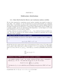
8 By using ( ) in the formp(x, y) =pX(x)p(y|x) for allx, y,( )it is possible to construct a bivariate distribution from two components: either marginal distribution and theconditional distribution of the other variable given the one whose marginal distribution is specified. Thuswhile marginal distributions are themselves insufficient to build a bivariate distribution , the conditionalprobability function captures exactly what additional information is Continuous Bivariate distribution of a pair of continuous random variablesXandYdefined on the same sample space(that is, in reference to the same experiment) is given formally by an extension of the device used in theunivariate case, a density function.

9 If we think of the pair (X, Y) as a random point in the plane, thebivariate probability density functionf(x, y) describes a surface in 3-dimensional space, and the probabilitythat (X, Y) falls in a region in the plane is given by the volume over that region and under the surfacef(x, y). Since volumes are given as double integrals, the rectangular region witha < X < bandc < Y < dhas probabilityP(a < X < bandc < Y < d) = dc baf(x, y)dxdy.( )[Figure ]It will necessarily be true of any bivariate density thatf(x, y) 0 for allx, y( )and f(x, y)dxdy= 1,( )that is, the total volume between the surfacef(x, y) and thex yplane is 1. Also, any functionf(x, y)satisfying ( ) and ( ) describes a continuous bivariate probability can help the intuition to think of a continuous bivariate distribution as a unit mass resting squarelyon the plane, not concentrated as spikes at a few separated points, as in the discrete case.

10 It is as if the massis made of a homogeneous substance, and the functionf(x, y) describes the upper surface of the we are given a bivariate probability densityf(x, y), then we can, as in the discrete case, calculate themarginal probability densitiesofXand ofY; they are given byfX(x) = f(x, y)dyfor allx,( )fY(y) = f(x, y)dxfor ally.( )Just as in the discrete case, these give the probability densities ofXandYconsidered separately, ascontinuous univariate random relationships ( ) and ( ) are rather close analogues to the formulae for the discrete case, ( )and ( ). They may be justified as follows: for anya < b, the events a < X b and a < X band < Y < are in fact two ways of describing the same event.