Chapter 3 Multivariate Probability

1 Chapter 3 Multivariate Joint Probability mass and density functionsRecall that a basic Probability distribution is defined overa random variable, and a randomvariable maps from the sample space to the real when you are interestedin the outcome of an event that is not naturally characterizable as a single real-valued number,such as the two formants of a vowel?The answer is simple: Probability mass and density functions can be generalized overmultiple random variables at once. If all the random variables are discrete, then they aregoverned by ajoint Probability mass function; if all the random variables are con-tinuous, then they are governed by ajoint Probability density function. There aremany things we ll have to say about the joint distribution ofcollections of random variableswhich hold equally whether the random variables are discrete, continuous, or a mix of these cases we will simply use the term joint density with the implicit understandingthat in some cases it is a Probability mass , for random variablesX1, X2, , XN, the joint density is written asp(X1=x1, X2=x2, , XN=xn)( )or simplyp(x1, x2, , xn)( )for some of the random variables are discrete and others are continuous, then technically it is a probabilitydensity function rather than a Probability mass function that they follow.

2 But whenever one is required tocompute the total Probability contained in some part of the range of the joint density, one must sum on thediscrete dimensions and integrate on the continuous Joint cumulative distribution functionsFor a single random variable, the cumulative distribution function is used to indicate theprobability of the outcome falling on a segment of the real number line. For a collection ofNrandom variablesX1, .. , XN(or density), the analogous notion is thejoint cumulativedistribution function, which is defined with respect to regions ofN-dimensional joint cumulative distribution function, which is sometimes notated asF(x1, , xn), isdefined as the Probability of the set of random variables all falling at or below the specifiedvalues ofXi:2F(x1, , xn)def=P(X1 x1, , XN xn)The natural thing to do is to use the joint cpd to describe the probabilities of rectangularvolumes.

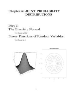
3 For example, supposeXis thef1formant andYis thef2formant of a givenutterance of a vowel. The Probability that the vowel will liein the region 480Hz f1 530Hz,940Hz f2 1020Hz is given below:P(480Hz f1 530Hz,940Hz f2 1020Hz) =F(530Hz,1020Hz) F(530Hz,940Hz) F(480Hz,1020Hz) +F(480Hz,940Hz)and visualized in Figure using the code MarginalizationOften we have direct access to a joint density function but weare more interested in theprobability of an outcome of a subset of the random variablesin the joint density. Obtainingthis Probability is calledmarginalization, and it involves taking a weighted sum3over thepossible outcomes of the random variables that are not of interest. For two variablesX, Y:2 Technically, the definition of the Multivariate cumulativedistribution function isF(x1, , xn)def=P(X1 x1, , XN xn) =X~x hx1, ,xNip(~x)[Discrete]( )F(x1, , xn)def=P(X1 x1, , XN xn) =Zx1 ZxN p(~x)dxN dx1[Continuous]( )3or integral in the continuous caseRoger Levy Probabilistic Models in the Study of Languagedraft, November 6, 2012382003004005006007008005001000150020 002500f1f2 Figure.

4 The Probability of the formants of a vowel landing in the grey rectangle can becalculated using the joint cumulative distribution (X=x) =XyP(x, y)=XyP(X=x|Y=y)P(y)In this caseP(X) is often called amarginal densityand the process of calculating it fromthe joint densityP(X, Y) is known an example, consider once again the historical English example of Section Wecan now recognize the table in I as giving the joint density over two binary-valued randomvariables: the position of the object with respect to the verb, which we can denote asX,and the pronominality of the object NP, which we can denote asY. From the joint densitygiven in that section we can calculate the marginal density ofX:P(X=x) =( + = + = ( )Additionally, if you now look at the old English example of Section and how wecalculated the denominator of Equation , you will see that it involved marginalizationover the animacy of the object NP.)

5 Repeating Bayes rule for reference:P(A|B) =P(B|A)P(A)P(B)It is very common to need to explicitly marginalize overAto obtain the marginal prob-ability forBin the computation of the denominator of the right-hand Levy Probabilistic Models in the Study of Languagedraft, November 6, Linearity of expectation, covariance, correlation,and variance f sums of random Linearity of the expectationLinearity of the expectation is an extremely important property and can expressed in twoparts. First, if yourescalea random variable, its expectation rescales in the exact same , ifY=a+bX, thenE(Y) =a+bE(X).Second, the expectation of the sum of random variables is thesum of the is, ifY=PiXi, thenE(Y) =PiE(Xi). This holds regardless of any conditionaldependencies that hold among can put together these two pieces to express the expectation of a linear combinationof random variables.

6 IfY=a+PibiXi, thenE(Y) =a+XibiE(Xi)( )This is incredibly convenient. We ll demonstrate this convenience when we introduc thebinomial distribution in Section CovarianceThecovariancebetween two random variablesXandYis a measure of how tightly theoutcomes ofXandYtend to pattern together. It defined as follows:Cov(X, Y) =E[(X E(X))(Y E(Y))]When the covariance is positive,Xtends to be high whenYis high, and vice versa; whenthe covariance is negative,Xtends to be high whenYis low, and vice a simple example of covariance we ll return once again to the Old English example ofSection ; we repeat the joint density for this example below, with the marginal densitiesin the row and column margins:(1)Coding forY01 Coding forXPronoun Not can compute the covariance by treating each ofXandYas a Bernoulli random variable,using arbitrary codings of 1 forPostverbalandNot Pronoun, and 0 forPreverbalandRoger Levy Probabilistic Models in the Study of Languagedraft, November 6, 201240 Pronoun.

7 As a result, we haveE(X) = ,E(Y) = The covariance between thetwo can then be computed as follows:(0 ) (0 .762) .224(for X=0,Y=0)+(1 ) (0 .762) (for X=1,Y=0)+(0 ) (1 .762) (for X=0,Y=1)+(1 ) (1 .762) (for X=1,Y=1)= conditionally independent given our state of knowledge, then Cov(X, Y)is zero (Exercise asks you to prove this). Covariance and scaling random variablesWhat happens toCov(X, Y) when you scaleX? LetZ=a+bX. It turns out that thecovariance withYincreases byb(Exercise asks you to prove this):Cov(Z, Y) =bCov(X, Y)As an important consequence of this, rescaling a random variable byZ=a+bXrescales itsvariance byb2: Var(Z) =b2 Var(X) (see Exercise ). CorrelationWe just saw that the covariance of word length with frequencywas much higher than withlog frequency.

8 However, the covariance cannot be compared directly across different pairs ofrandom variables, because we also saw that random variableson different scales ( , thosewith larger versus smaller ranges) have different covariances due to the scale. For this reason,it is commmon to use thecorrelation as a standardized form of covariance: XY=Cov(X, Y)pV ar(X)V ar(Y)[1] the word order & pronominality example above, where we found that the covarianceof verb-object word order and object pronominality was , we can re-express this rela-tionship as a correlation. We recall that the variance of a Bernoulli random variable withsuccess parameter is (1 ), so that verb-object word order has variance and objectpronominality has variance The correlation between the two random variables is independent, then their covariance (and hence correlation) is Levy Probabilistic Models in the Study of Languagedraft, November 6, Variance of the sum of random variablesIt is quite often useful to understand how the variance of a sum of random variables isdependent on their joint distribution .

9 LetZ=X1+ +Xn. ThenVar(Z) =nXi=1 Var(Xi) +Xi6=jCov(Xi, Xj)( )Since the covariance between conditionally independent random variables is zero, it followsthat the variance of the sum of pairwise independent random variables is the sum of The binomial distributionWe re now in a position to introduce one of the most importantprobability distributions forlinguistics, thebinomial distribution . The binomial distribution family is characterizedby two parameters,nand , and a binomially distributed random variableYis defined asthe sum ofnidentical, independently distributed ( ) Bernoullirandom variables, eachwith parameter .For example, it is intuitively obvious that the mean of a binomially distributed parametersnand is n. However, it takes some work to show this explicitly bysumming over the possible outcomes ofYand their probabilities.

10 On the other hand,Ycan be re-expressed as the sum ofnBernoulli random variablesXi. The resultingprobability density function is, fork= 0,1, .. , n:4P(Y=k) = nk k(1 )n k( )We ll also illustrate the utility of the linearity of expectation by deriving the expectationofY. The mean of eachXiis trivially , so we have:E(Y) =nXiE(Xi)( )=nXi = n( )which makes intuitive , since a binomial random variable is the sum ofnmutually independent Bernoullirandom variables and the variance of a Bernoulli random variable is (1 ), the varianceof a binomial random variable isn (1 ).4 Note that nk is pronounced nchoosek , and is defined asn!k!(n k)!. In turn,n! is pronounced nfactorial , and is defined asn (n 1) 1 forn= 1,2, .., and as 1 forn= Levy Probabilistic Models in the Study of Languagedraft, November 6, The multinomial distributionThemultinomial distributionis the generalization of the binomial distribution tor 2possible outcomes.