Transcription of Chapter 3 State Variable Models - Engineering
1 1 Chapter 3 State Variable ModelsThe State Variables of a Dynamic SystemThe State Differential EquationSignal-Flow Graph State VariablesThe Transfer Function from the State Equation2 Introduction In the previous Chapter , we used Laplace transform to obtain the transfer function Models representing linear, time-invariant, physical systems utilizing block diagrams to interconnect systems. In Chapter 3, we turn to an alternative method of system modeling using time-domain methods.
2 In Chapter 3, we will consider physical systems described by an nth-order ordinary differential equations. Utilizing a set of variables known as State variables, we can obtain a set of first-order differential equations. The time-domain State Variable model lends itself easily to computer solution and Control System With the ready availability of digital computers, it is convenient to consider the time-domain formulation of the equations representing control systems.
3 The time-domain is the mathematical domain that incorporates the response and description of a system in terms of time t. The time-domain techniques can be utilized for nonlinear, time-varying, and multivariable systems (a system with several input and output signals). A time-varying control system is a system for which one or more of the parameters of the system may vary as a function of time. For example, the mass of a missile varies as a function of time as the fuel is expended during flight4 Terms State :The State of a dynamic system is the smallest set of variables (called State variables) so that the knowledge of these variables at t= t0, together with the knowledge of the input for t t0, determines the behavior of the system for any time t t0.
4 State Variables:The State variables of a dynamic system are the variables making up the smallest set of variables that determine the State of the dynamic system. State Vector:If nstate variables are needed to describe the behavior of a given system, then the nstate variables can be considered the ncomponents of a vector x. Such vector is called a State vector. State Space:The n-dimensional space whose coordinates axes consist of the x1axis, x2axis, .., xnaxis, where x1, x2.
5 , xnare State variables, is called a State space. State -Space Equations:In State -space analysis, we are concerned with three types of variables that are involved in the modeling of dynamic system: input variables, output variables, and State State Variables of a Dynamic System The State of a system is a set of variables such that the knowledge of these variables and the input functions will, with the equations describing the dynamics, provide the future State and output of the system.
6 For a dynamic system, the State of a system is described in terms of a set of State (t)u2(t)y1(t)y2(t)Input SignalsOutput Signals6 State Variables of a Dynamic SystemDynamic SystemState x(t)u(t) Inputy(t) Outputx(0) initial conditiondynamics thedescribing equations theand inputs, excitation thestate,present given the system, a of response future thedescribe variablesstate The7 The State Differential EquationThe State of a system is described by the set of first-order differential equations written in terms of the State variables (x1, x2.)
7 , xn)equation) aldifferenti (StateBu Axx.+=signals)output -equation(Output Du Cxy+=matrix nsmission direct tra :D matrix;Output :Cmatrixinput :B matrix; State :A + = ++++++=++++++=++++++= .. Budtdxx=&8 Block Diagram of the Linear, Continuous Time Control System)( (t) dtC(t)D(t)u(t)y(t)A(t))(u )D()( x)C()()(u )B()x(t)A()( +=+=++++x(t)9 Mass Grounded, M(kg)Mechanical system described by the first-order differential equationFa(t)x (t) ===ttaadttFMtvdttxdMdtdvMtFtxtvtT0)(1)() ()((m) )(position Linear (m/sec) )(ocity Linear velm)-(N )( torqueAppied22av (t)M10 Mechanical Example.
8 Mass-Spring DamperA set of State variables sufficient to describe this system includes the position and the velocity of the mass, therefore, we will define a set of State variables as (x1, x2)uMxMkxmbdtdxxdtdxtukxbxdtdxMtukydtdyb dtydMdttdytxtytx1 ;)()()()()()(122211222221+ ===++=++==MKbWall frictiony(t)u(t)constant Spring :k11 Example 1:Consider the previous mechanical system. Assume that the system is linear. The external force u(t) is the input to the system, and the displacement y(t) of the mass is the output.
9 The displacement y(t) is measured from the equilibrium position in the absence of the external force. This system is a single-input-single-output system.[][]0 ,0 1C ,10B ,- -1 0 AuCxy ;BAxx:form standard in the areequation output theandequation State TheEquation)(Output 0 1 Equation) ( State 1021 mb- mk-1 0have weform,matrix vector aIn :isequation output The1 then );()();()()( and )( : variables twodefine usLet twoinvolvesit meansIt second a is = =+=+= = + = =+ =====++DmmbmkDuxxyumxxxxxyumxmbxmkxxxtyt xtytxtxtxukyybym12 Electrical and Mechanical CounterpartsResistorRi2 Damper / Cv2 Gravity.
10 Li2 Mass / mv2/ j 2 Kinetic ElectricalMechanicalEnergy13 Resistance, R(ohm)v(t)Ri(t))(1)()()()(Current )( voltageAppiedtvRtitRitvtitv==14 Inductance, L(H)v(t)Li(t) ==ttdttvLtidttdiLtvtitv0)(1)()()()(Curre nt )( voltageAppied15 Capacitance, C(F)v(t)Ci(t)dttdvCtidttiCtvtitvtt)()()( 1)()(Current )( voltageAppied0== 16 Electrical Example: An RLCC ircuitCLRu(t)iLiCvC() ()212122102012221)()( : thenis signaloutput The1)(11 )( :by drepresente is system theofoutput The)(junction at the KCL USEnetwork theofenergy initial total theis )( and )(2/12/1)( ).