Chapter 4. SAMPLING DISTRIBUTIONS

1 Chapter 4. SAMPLING DISTRIBUTIONS . In agricultural research, we commonly take a number of plots or animals for experimental use. In effect we are working with a number of individuals drawn from a large population. Usually we don't know the exact characteristics of the parent population from which the plots or animals are drawn. Hopefully the samples we draw and the statistics we compute from them are close approximations of the parameters of the parent populations. To ensure a representative sample we use the principle of randomization. A random sample is one drawn so that each individual in the population has the same chance of being included.

2 The parameters of a population are based on all of its variates and are therefore fixed. The statistics vary from sample to sample. Therefore the possible values of a statistic constitute a new population, a distribution of the sample statistic. distribution of Sample Means Consider a population of N variates with mean and standard deviation , and draw all possible samples of r variates. Assume that the samples have been replaced before each drawing, so that the total number of different samples which can be drawn is the combination of N things taken r at a time, that is N. M = ( r ). The mean of all these sample means ( Y1 , Y2.)

3 , YM ) is denoted by y and their standard deviation by y , also known as the standard error of a mean. The mean of the sample means is the same as the mean of the parent population, , y = Yi / M = = Yi / N. 2. The variance of the sample means ( y ) equals the variance of the parent ( 2) population divided by the sample size (r) and multiplied by a factor f. 2. y = ( Yi y ) 2 / M = ( 2 / r ) f where f = (N - r) / (N - 1). Note that the standard error of a mean approaches the standard deviation of the parent population divided by the square root of the sample size, y = / r for a large population ( , f approaches unity). The larger the size of a sample, the smaller the variance of the sample mean.

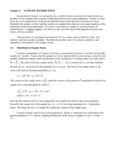
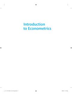
4 Consider samples taken from a normal population. Figure 4-1 illustrates the relationship of the parent population (r = 1) with the SAMPLING DISTRIBUTIONS of the means of samples of size r = 8 and r =. 16. Figure 4-1. Figure 4-2. The relation of the frequencies of means for r = 3 from the population 1,2,3,4,5,6,7 and the normal distribution . Even when the variates of the parent population are not normally distributed, the means generated by samples tend to be normally distributed. This can be illustrated by considering samples of size 3 from a simple non-normal population with variates 1,2,3,4,5,6, and 7. Table 4-1 presents all possible sample means, and Figure 4-2 shows the frequency distribution of the means which approaches the normal frequency curve.

5 Table 4-1. All possible different samples of size 3 from the population 1, 2, 3, 4, 5, 6, 7 with = 4 and = 2. Sample No. Sample Y Sample No. Sample 1 1 2 3 2 19 2 3 7 4. 2 1 2 4 2 1/3 20 2 4 5 3 2/3. 3 1 2 5 2 2/3 21 2 4 6 4. 4 1 2 6 3 22 2 4 7 4 1/3. 5 1 2 7 3 1/3 23 2 5 6 4 1/3. 6 1 3 4 2 2/3 24 2 5 7 4 2/3. 7 1 3 5 3 25 2 6 7 5. 8 1 3 6 3 1/3 26 3 4 5 4. 9 1 3 7 3 2/3 27 3 4 6 4 1/3. 10 1 4 5 3 1/3 28 3 4 7 4 2/3. 11 1 4 6 3 2/3 29 3 5 6 4 2/3. 12 1 4 7 4 30 3 5 7 5. 13 1 5 6 4 31 3 6 7 5 1/3. 14 1 5 7 4 1/3 32 4 5 6 5. 15 1 6 7 4 2/3 33 4 5 7 5 1/3. 16 2 3 4 3 34 4 6 7 5 2/3. 17 2 3 5 3 1/3 35 5 6 7 6. 18 2 3 6 3 2/3. The mean and standard deviation of the distribution of the sample means are: 1.

6 Y = ( 2 + 21 / 3 + 2 2 / 3+..+52 / 3 + 6) = 4 = . 35. 2 1. y = {( 2 4 ) 2 + ( 21 / 3 4 ) 2 +..+ (52 / 3 4 ) 2. 35. 2 N r 4 4 8. + (6 4)2 } = ( ) = ( ) =. r N 1 3 6 9. y = 8 / 9. Note that in this particular case, we have used a simple population with only seven elements. Sample means from samples with increasing size, from a large population will more closely approach the normal curve. This tendency of sample means to approach a normal distribution with increasing sample size is called the central limit theorem. The distribution of Sample Mean Differences In section we mentioned that the means of all possible samples of a given size (r1) drawn 2 2.

7 From a large population of Y's are approximately normally distributed with y = y and y = y / r1 . Now consider drawing samples of size r2 from another large population, X's. The parameters of these 2 2. sample means are also approximately normally distributed with x = x and x = x / r2 . An additional approximately normal population is generated by taking differences between all possible 2. means, Y X = d , with the parameters d and . d d = y x = y x and 2 2 2 2 2. = y + x = y / r1 + x / r2. d When the variances of the parent populations are equal, 2 2 2. y = x (= 2 ) and sample sizes are the same, r = r1 = r2 then = 2 2 / r . d The square root of the variance of mean differences, d , is usually called the standard error of the difference between sample means.

8 Figure 4-3 diagrams the generation of a population of mean differences by repeated SAMPLING from two populations of individual variates and indicates relationships among the parameters. The relationships among the population parameters developed in Sections 4-1 and 4-2 are important in statistical evaluation. With information about the parent population one can estimate parameters associated with a sample mean or the difference between two sample means. This will be discussed further in later chapters. Figure 4-3. Relationships between parameters of a population of sample mean differences and parent populations. Normal Approximation to Binomial Although a formula is given in Chapter 3 to calculate probabilities for binomial events, if the number of trials (n) is large the calculations become tedious.

9 Since many practical problems involve large samples of repeated trials, it is important to have a more rapid method of finding binomial probabilities. It was also pointed out in Chapter 3 that the normal distribution is useful as a close approximation to many discrete DISTRIBUTIONS when the sample size is large. When n > 30, the sample is usually considered large. In this section we will show how the normal distribution is used to approximate a binomial distribution for ease in the calculation of probabilities. Since the normal frequency curve is always symmetric, whereas the binomial histogram is symmetric only when p = q = 1/2, it is clear that the normal curve is a better approximation of the binomial histogram if both p and q are equal to or nearly equal to 1/2.

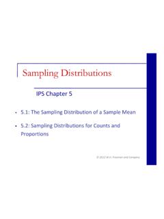
10 The more p and q differ from 1/2, the greater the number of trials are required for a close approximation. Figure 4-4 shows how closely a normal curve can approximate a binomial distribution with n = 10 and p = q = 1/2. Figure 4-5 illustrates a case where the normal distribution closely approximates the binomial when p is small but the sample size is large. Figure 4-4. Binomial distribution for p = and n = 10. Figure 4-5. Binomial distribution for p = and n = 100. To use the normal curve to approximate discrete binomial probabilities, the area under the curve must include the area of the block of the histogram at any value of r, the number of occurrences under consideration.