Transcription of Chapter 6 - Random Processes
1 EE385 Class Notes 11/11/2014 John Stensby Updates at 6-1 Chapter 6 - Random Processes Recall that a Random variable X is a mapping between the sample space S and the extended real line R+. That is, X : S R+. A Random process ( stochastic process) is a mapping from the sample space into an ensemble of time functions (known as sample functions). To every S, there corresponds a function of time (a sample function) X(t; ). This is illustrated by Figure 6-1. Often, from the notation, we drop the variable , and write just X(t). However, the sample space variable is always there, even if it is not shown explicitly. For a fixed t = t0, the quantity X(t0; ) is a Random variable mapping sample space S into the real line.
2 For fixed 0 S, the quantity X(t; 0) is a well-defined, non- Random , function of time. Finally, for fixed t0 and 0, the quantity X(t0; 0) is a real number. Example 6-1: X maps Heads and Tails Consider the coin tossing experiment where S = {H, T}. Define the Random function X(t;Heads) = sin(t) X(t;Tails) = cos(t) timeX(t; 1)X(t; 2)X(t; 3)X(t; 4)Figure 6-1: Sample functions of a Random process. EE385 Class Notes 11/11/2014 John Stensby Updates at 6-2 Continuous and Discrete Random Processes For a continuous Random process, probabilistic variable takes on a continuum of values. For every fixed value t = t0 of time, X(t0; ) is a continuous Random variable . Example 6-2: Let Random variable A be uniform in [0, 1]. Define the continuous Random process X(t; ) = A( )s(t), where s(t) is a unit-amplitude, T-periodic square wave.
3 Notice that sample functions contain periodically-spaced (in time) jump discontinuities. However, the process is continuous. For a discrete Random process, probabilistic variable takes on only discrete values. For every fixed value t = t0 of time, X(t0; ) is a discrete Random variable . Example 6-3: Consider the coin tossing experiment with S = {H, T}. Then X(t;H) = sin(t), X(t;T) = cos(t) defines a discrete Random process. Notice that the sample functions are continuous functions of time. However, the process is discrete. Distribution and Density Functions The first-order distribution function is defined as F(x,t) = P[X(t) x]. (6-1) The first-order density function is defined as fxtdF(x,(;) t) dx.
4 (6-2) These definitions generalize to the nth-order case. For any given positive integer n, let x1, x2, .. , xn denote n realization variables, and let t1, t2, .. , tn denote n time variables. Then, define the nth-order distribution function as F(x1, x2, .. , xn; t1, t2, .. , tn ) = P[X(t1) x1, X(t2) x2, .. , X(tn) xn]. (6-3) EE385 Class Notes 11/11/2014 John Stensby Updates at 6-3 Similarly, define the nth-order density function as fn(x , x , .. , x ; t , t.)
5 , t ) = F(x , x , .. , x ; t , t , .. , t ) xx .. x12n12n12n12n12n (6-4) In general, a complete statistical description of a Random process requires knowledge of all order distribution functions. Stationary Random Process A process X(t) is said to be stationary if its statistical properties do not change with time. More precisely, process X(t) is stationary if F(x1, x2, .. , xn; t1, t2, .. , tn) = F(x1, x2, .. , xn; t1+c, t2+c, .. , tn+c) (6-5) for all orders n and all time shifts c. Stationarity influences the form of the first- and second-order distribution/density functions. Let X(t) be stationary, so that F(x; t) = F(x; t+c) (6-6) for all c.
6 This implies that the first-order distribution function is independent of time. A similar statement can be made concerning the first-order density function. Now, consider the second-order distribution F(x1,x2;t1,t2) of stationary X(t); for all t1, t2 and c, this function has the property 1212121212121122F(x , x ; t , t ) = F(x , x ; t + c, t + c) = F(x , x ; 0, + ) if c = twherett .= F(x , x ; , 0 ) if c = t (6-7) EE385 Class Notes 11/11/2014 John Stensby Updates at 6-4 Equation (6-7) must be true for all t1, t2 and c. Hence, the second-order distribution cannot depend on absolute t1 and t2; instead, F(x1,x2;t1,t2) depends on the time difference t2 t1.
7 In F(x1,x2;t1,t2), you will only see t1 and t2 appear together as t2 t1, which we define as . Often, for stationary Processes , we change the notation and define " new " notation" old " notation121211F(x , x ; )F(x , x ; t , t + ) . (6-8) Similar statements can be made concerning the second-order density function. Be careful! These conditions on first-order F(x) and second-order F(x1, x2; ) are necessary conditions; they are not sufficient to imply stationarity. For a given Random process, suppose that the first order distribution/density is independent of time and the second-order distribution/density depends only on the time difference.
8 Based on this knowledge alone, we cannot conclude that X(t) is stationary. First- and Second-Order Probabilistic Averages First- and second-order statistical averages are useful. The expected value of general Random process X(t) is defined as (t) = E[X(t)] = x f(x; t) dx- z. (6-9) In general, this is a time-varying quantity. The expected value is often called a first-order statistic since it depends on a first-order density function. The autocorrelation function of X(t) is defined as Rt tEXt Xtxx fx x t t dxdx(, ) [()( )]( , ;, )121212 1 2121 2 zz. (6-10) In general, R depends on two time variables, t1 and t2.
9 Also, R is an example of a second-order EE385 Class Notes 11/11/2014 John Stensby Updates at 6-5 statistic since it depends on a second-order density function. Suppose X(t) is stationary. Then the mean = E[X(t)] = x f(x) dx- z (6-11) is constant, and the autocorrelation function REXtXtxxfxxdxdx() [()()]( , ;) zz121 21 2 (6-12) depends only on the time difference = t2 t1 (it does not depend on absolute time). However, the converse is not true: the conditions a constant and R( ) independent of absolute time do not imply that X(t) is stationary.
10 Wide Sense Stationarity (WSS) Process X(t) is said to be wide-sense stationary (WSS) if 1) Mean = E[X(t)] is constant, and 2) Autocorrelation R( ) = E[X(t)X(t+ )] depends only on the time difference. Note that stationarity implies wide-sense stationarity. However, the converse is not true: WSS does not imply stationarity. Ergodic Processes A process is said to be Ergodic if all orders of statistical and time averages are interchangeable. The mean, autocorrelation and other statistics can be computed by using any sample function of the process. That is zzzzzEX txf xTXt dtREXtXtxxfxx dxTXtXtdtTTTTTT[()]()dx()()[ () ()]( , ;)dx() () .limitlimit1212121 21 2 (6-13) EE385 Class Notes 11/11/2014 John Stensby Updates at 6-6 This idea extends to higher-order averages as well.