Transcription of Chapter 9 Multirate Digital Signal Processing
1 EEE305 , EEE801 Part A : Digital Signal Processing Chapter 9: Multirate Digital Signal Processing University of Newcastle upon Tyne Page Chapter 9 Multirate Digital Signal Processing Introduction Multirate systems have gained popularity since the early 1980s and they are commonly used for audio and video Processing , communications systems, and transform analysis to name but a few. In most applications Multirate systems are used to improve the performance, or for increased computational efficiency. The two basic operations in a Multirate system are decreasing (decimation) and increasing (interpolation) the sampling-rate of a Signal . Multirate systems are sometimes used for sampling-rate conversion, which involves both decimation and interpolation. Decimation Decimation can be regarded as the discrete-time counterpart of sampling.
2 Whereas in sampling we start with a continuous-time Signal x(t) and convert it into a sequence of samples x[n], in decimation we start with a discrete-time Signal x[n] and convert it into another discrete-time Signal y[n], which consists of sub-samples of x[n]. Thus, the formal definition of M-fold decimation, or down-sampling, is defined by Equation In decimation, the sampling rate is reduced from Fs to Fs/M by discarding M 1 samples for every M samples in the original sequence. = ==kknMxkhnMvny][][][][ ( ) h[k] Digital anti-aliasingfilter M Sampling-rate compressor x[n] y[n]Fs Fs/M v[n] Figure : Block diagram notation of decimation, by a factor of M. The block diagram notation of the decimation process is depicted in Figure An anti-aliasing Digital filter precedes the down-sampler to prevent aliasing from occurring, due to the lower sampling rate.
3 The subject of aliasing in decimated signals is covered in more detail in Section In Figure below, it illustrates the concept of 3-fold decimation M = 3. Here, the samples of x[n] corresponding to n = .., -2, 1, 4,.. and n = .., -1, 2, 5,.. are lost in the decimation process. In general, the samples of x[n] corresponding to n kM, where k is an integer, are discarded in M-fold decimation. In Figure (b), it shows samples of the decimated Signal y[n] spaced three times wider than the samples of x[n]. This is not a coincidence. In real time, the decimated Signal appears at a slower rate than that of the original Signal by a factor of M. If the sampling frequency of x[n] is Fs, then that of y[n] is Fs/M. Interpolation Interpolation is the exact opposite of decimation. It is an information preserving operation, in that all samples of x[n] are present in the expanded Signal y[n].
4 The mathematical definition of L-fold interpolation is defined by Equation and the block diagram notation is depicted in Figure Interpolation works by inserting (L 1) zero-valued samples for each input sample. The sampling rate therefore increases from Fs to LFs. With reference to Figure , the expansion process is followed by a unique Digital low-pass filter called an anti-imaging filter. Although the expansion process does not cause aliasing in the interpolated Signal , it does however yield undesirable replicas in the Signal s frequency spectrum. We shall see how this special filter, in Section , is necessary to remove these replicas from the frequency spectrum. = =kknwkhLny][][][ ( ) EEE305 , EEE801 Part A : Digital Signal Processing Chapter 9: Multirate Digital Signal Processing University of Newcastle upon Tyne Page Where, =integer-non is L if , 0integeran is L if, ]/[][nnLnxnw In Figure below, it depicts 3-fold interpolation of the Signal x[n] L = 3.
5 The insertion of zeros effectively attenuates the Signal by L, so the output of the anti-imaging filter must be multiplied by L, to maintain the same Signal magnitude. (a)nx[n] (b)ny[n] Figure : Decimation of a discrete-time Signal by a factor of 3. L Sampling-rate expanderh[k] Anti-imaging filter x[n] y[n]Fs LFs w[n] Figure : Block diagram notation of interpolation, by a factor of L. Frequency Transforms of Decimated and Expanded Sequences The analysis of decimation and expansion is better understood by assessing their respective frequency spectrums using the Fourier transform. Decimation The implications of aliasing caused by decimation are very similar to those in the case of sampling a continuous-time Signal , in Section In general, if the Fourier transform of a Signal , X( ), occupies the entire bandwidth from [- , ], then the Fourier transform of the decimated Signal , X( M)( ), will be aliased.
6 This is due to the superposition of the M shifted and frequency-scaled transforms. This is illustrated in Figure below, which shows the aliasing phenomenon for M = 3. EEE305 , EEE801 Part A : Digital Signal Processing Chapter 9: Multirate Digital Signal Processing University of Newcastle upon Tyne Page (a)nx[n] (b)ny[n] Figure : Interpolation of a discrete-time Signal by a factor of 3. - X( )3 (a) -3 - Y( ) 3 (c) -3 - V( )3 (b) -3 Figure : Aliasing caused by decimation; (a) Fourier transform of the original Signal ; (b) After decimation filtering; (c) Fourier transform of the decimated Signal . In Figure (a) it shows the Fourier transform of the original Signal . Part (b) shows the Signal after lowpass filtering. In Figure (c), it depicts the expanded spectrum after decimation. EEE305 , EEE801 Part A : Digital Signal Processing Chapter 9: Multirate Digital Signal Processing University of Newcastle upon Tyne Page Expansion The effect of expansion on a Signal in the frequency domain is illustrated in Figure below.
7 Part (a) shows the Fourier transform of the original Signal ; part (b) illustrates the Fourier transform of the Signal with zeros added W( ); and part (c) shows the Fourier transform of the Signal after the interpolation filter. It is clearly visible that the shape of the Fourier transform is compressed by a factor L in the frequency axis and is also repeated L times in the range of [- , ]. Despite the compression of the Signal in the frequency axis, the shape of the Fourier transform is still preserved, confirming that expansion does not lead to aliasing. These replicas are removed by a Digital low-pass filter called an anti-imaging filter, as indicated in Figure X( ) (a) - /3- /3 W( ) (b) - /3- /3 Y( ) (c) - Figure : Expansion in the frequency domain of the original Signal (a) and the expanded Signal (b).
8 Sampling-rate Conversion A common use of Multirate Signal Processing is for sampling-rate conversion. Suppose a Digital Signal x[n] is sampled at an interval T1, and we wish to obtain a Signal y[n] sampled at an interval T2. Then the techniques of decimation and interpolation enable this operation, providing the ratio T1/T2 is a rational number L/M. Sampling-rate conversion can be accomplished by L-fold expansion, followed by low-pass filtering and then M-fold decimation, as depicted in Figure It is important to emphasis that the interpolation should be performed first and decimation second, to preserve the desired spectral characteristics of x[n]. Furthermore by cascading the two in this manner, both of the filters can be combined into one single low-pass filter. EEE305 , EEE801 Part A : Digital Signal Processing Chapter 9: Multirate Digital Signal Processing University of Newcastle upon Tyne Page L Sampling-rate expander h[k] Low-pass filter x[n] y[n] Fs LFs M Sampling-rate compressorLFs LFs/M Figure : Sampling-rate conversion by expansion, filtering, and decimation.
9 An example of sampling-rate conversion would take place when data from a CD is transferred onto a DAT. Here the sampling-rate is increased from kHz to 48 kHz. To enable this process the non-integer factor has to be approximated by a rational number: Hence, the sampling-rate conversion is achieved by interpolating by L from kHz to [ ] = 7056 kHz. Then decimating by M from 7056 kHz to [7056/147] = 48 kHz. Multistage Approach When the sampling-rate changes are large, it is often better to perform the operation in multiple stages, where Mi(Li), an integer, is the factor for the stage i. M = or L = An example of the multistage approach for decimation is shown in Figure The multistage approach allows a significant relaxation of the anti-alias and anti-imaging filters, with a consequent reduction in the filter complexity.
10 The optimum number of stages is one that leads to the least computational effort in terms of either the multiplications per second (MPS), or the total storage requirement (TSR). x[n] y[n] Fs 11 MLFs 2211 MLMLFs M1 h1[k] Stage 1 L1 M2 h1[k] Stage 2 L2 Figure : Multistage approach for the decimation process. Polyphase Filters Potential computational savings can be made within the process of decimation, interpolation, and sampling-rate conversion. Polyphase filters is the name given to certain realisations of Multirate filtering operations, which facilitate computational savings in both hardware and software. As an example, the combined low-pass filter in the sampling-rate converter, as illustrated in Figure , can be re-drawn as a realisation structure ( Chapter 3). In principle, the simplest realisation of the low-pass filter is the direct-form FIR structure, as depicted in Figure However, this type of structure is very inefficient owing to the interpolation process, which introduces (L 1) zeros between consecutive points in the Signal .