Transcription of CHAPTER 9: SERIAL CORRELATION
1 CHAPTER 9: SERIAL CORRELATION Page 1 of 19 SERIAL CORRELATION (or autocorrelation) is the violation of Assumption 4 (observations of the error term are uncorrelated with each other). Pure SERIAL CORRELATION This type of CORRELATION tends to be seen in time series data. To denote a time series data set we will use a subscript. This type of SERIAL CORRELATION occurs when the error in one period is correlated with the errors in other periods. The model is assumed to be correctly specified. The most common form of SERIAL CORRELATION is called first-order SERIAL CORRELATION in which the error in time is related to the previous ( 1 period s error: , 1 1 The new parameter is called the first-order autocorrelation coefficient.)
2 The process for the error term is referred to as a first-order autoregressive process or AR(1). CHAPTER 9: SERIAL CORRELATION Page 2 of 19 The magnitude of tells us about the strength of the SERIAL CORRELATION and the sign indicates the nature of the SERIAL CORRELATION . 0 indicates no SERIAL CORRELATION 0 indicates positive SERIAL CORRELATION the error terms will tend to have the same sign from one period to the next CHAPTER 9: SERIAL CORRELATION Page 3 of 19 0 indicates negative SERIAL CORRELATION the error terms will tend to have a different sign from one period to the next CHAPTER 9: SERIAL CORRELATION Page 4 of 19 Impure SERIAL CORRELATION This type of SERIAL CORRELATION is caused by a specification error such as an omitted variable or ignoring nonlinearities.
3 Suppose the true regression equation is given by but in our model we do not include . The error term will capture the effect of . Since many economic variables exhibit trends over time, is likely to depend on , , , ,.. This will translate into a seeming CORRELATION between and , ,.. and this SERIAL CORRELATION would violate Assumption 4. CHAPTER 9: SERIAL CORRELATION Page 5 of 19 CHAPTER 9: SERIAL CORRELATION Page 6 of 19 A specification error of the functional form can also cause this type of SERIAL CORRELATION . Suppose the true regression equation between Y and X is quadratic but we assume it s linear. The error term will depend on . CHAPTER 9: SERIAL CORRELATION Page 7 of 19 The Consequences of SERIAL CORRELATION 1.
4 Pure SERIAL CORRELATION does not cause bias in the regression coefficient estimates. 2. SERIAL CORRELATION causes OLS to no longer be a minimum variance estimator. 3. SERIAL CORRELATION causes the estimated variances of the regression coefficients to be biased, leading to unreliable hypothesis testing. The t-statistics will actually appear to be more significant than they really are. CHAPTER 9: SERIAL CORRELATION Page 8 of 19 Testing for First-Order SERIAL CORRELATION Plotting the residuals is always a good first step. The most common formal test is the Durbin-Watson d test. The Durbin-Watson Test Consider the regression equation .. We are interested in determining if there is first-order autocorrelation in the error term , where is not autocorrelated.
5 CHAPTER 9: SERIAL CORRELATION Page 9 of 19 The test of the null hypothesis of no autocorrelation ( 0 ) is based on the Durbin-Watson statistic where the s are the residuals from the regression equation estimated by least squares. The value of this statistic is automatically reported in EViews regression output. Let s consider a few cases: Extreme positive CORRELATION Extreme negative CORRELATION No SERIAL CORRELATION CHAPTER 9: SERIAL CORRELATION Page 10 of 19 For an alternative of positive autocorrelation, : 0, look up the critical values in tables B-4, B-5 or B-6. The decision rule is as follows: Reject if . Do not reject if . Test inconclusive if . CHAPTER 9: SERIAL CORRELATION Page 11 of 19 Remedies for SERIAL CORRELATION 1.
6 Cochrane-Orcutt Procedure Transform the equation with AR(1) error structure .. , into one that is not autocorrelated. Consider the same model in period 1: Multiply both sides of this equation by : CHAPTER 9: SERIAL CORRELATION Page 12 of 19 Subtract this equation from the original equation: If were known, we could use OLS to obtain estimates that are BLUE. Unfortunately is not known and therefore must be estimated. CHAPTER 9: SERIAL CORRELATION Page 13 of 19 Step 1: Compute the residuals from the OLS estimation of .. Step 2: Estimate the first-order SERIAL CORRELATION coefficient using . Call this estimate.
7 Step 3: Transform the variables: , , , etc. Step 4: Regress on a constant, , ,.., and obtain the OLS estimates of the transformed equation. Step 5: Use these estimates to obtain a new set of estimates for the residual and then go back to Step 2. Step 6: This iterative procedure is stopped when the estimates of differ by no more than some pre-specified amount (eg. ) in two successive iterations. CHAPTER 9: SERIAL CORRELATION Page 14 of 19 2. Newey-West Standard Errors Adjust the standard errors of the estimated regression coefficients but not the estimates themselves since they are still unbiased. CHAPTER 9: SERIAL CORRELATION Page 15 of 19 Example Let s examine the relationship between Microsoft s marketing and advertising expenditures and its revenues.
8 Revenues marketing REVENUES: Microsoft s revenues in millions of dollars MARKETING: Microsoft s expenditures on marketing and advertising in millions of dollars Data: real data from Microsoft s website for 1987 through to 1999 Dependent Variable: REVENUES Method: Least Squares Sample: 1 13 Included observations: 13 Variable CoefficientStd. Errort-StatisticProb. MARKETING Mean dependent var R-squared dependent var of regression Akaike info criterion squared resid Schwarz criterion likelihood F-statistic stat Prob(F-statistic) CHAPTER 9: SERIAL CORRELATION Page 16 of 19 Plot of residuals against year.
9 -400-2000200400-100001000200030004000246 81012 ResidualActualFitted-400-300-200-1000100 20030040019841988199219962000 YEARRESIDCHAPTER 9: SERIAL CORRELATION Page 17 of 19 CHAPTER 9: SERIAL CORRELATION Page 18 of 19 Cochrane-Orcutt Procedure Dependent Variable: REVENUES Method: Least Squares Sample(adjusted): 2 13 Included observations: 12 after adjusting endpoints Convergence achieved after 52 iterations Variable CoefficientStd. Errort-StatisticProb. MARKETING (1) Mean dependent var R-squared dependent var of regression Akaike info criterion squared resid Schwarz criterion likelihood F-statistic stat Prob(F-statistic) AR Roots.
10 73 CHAPTER 9: SERIAL CORRELATION Page 19 of 19 Newey-West Standard Errors Dependent Variable: REVENUES Method: Least Squares Sample: 1 13 Included observations: 13 White Heteroskedasticity-Consistent Standard Errors & Covariance Variable CoefficientStd. Errort-StatisticProb. MARKETING Mean dependent var R-squared dependent var of regression Akaike info criterion squared resid Schwarz criterion likelihood F-statistic stat Prob(F-statistic)