Transcription of Chun-Lin, Liu February 23, 2010 - 國立臺灣大學
1 A Tutorial of the Wavelet TransformChun-Lin, LiuFebruary 23, 2010 Chapter IntroductionThe Fourier transform is an useful tool to analyze the frequency componentsof the signal. However, if we take the Fourier transform over the whole timeaxis, we cannot tell at what instant a particular frequency rises. Short-timeFourier transform (STFT) uses a sliding window to find spectrogram, whichgives the information of both time and frequency. But still another problemexists: The length of window limits the resolution in frequency.
2 Wavelettransform seems to be a solution to the problem above. Wavelet transformsare based on small wavelets with limited duration. The translated-versionwavelets locate where we concern. Whereas the scaled-version wavelets allowus to analyze the signal in different HistoryThe first literature that relates to the wavelet transform is Haar wavelet. Itwas proposed by the mathematician Alfrd Haar in 1909. However, the con-cept of the wavelet did not exist at that time. Until 1981, the concept wasproposed by the geophysicist Jean Morlet.
3 Afterward, Morlet and the physi-cist Alex Grossman invented the term wavelet in 1984. Before 1985, Haarwavelet was the only orthogonal wavelet people know. A lot of researcherseven thought that there was no orthogonal wavelet except Haar wavelet. For-tunately, the mathematician Yves Meyer constructed the second orthogonalwavelet called Meyer wavelet in 1985. As more and more scholars joined inthis field, the 1st international conference was held in France in 1988, Stephane Mallat and Meyer proposed the concept of multireso-lution.
4 In the same year, Ingrid Daubechies found a systematical method toconstruct the compact support orthogonal wavelet. In 1989, Mallat proposedthe fast wavelet transform . With the appearance of this fast algorithm, thewavelet transform had numerous applications in the signal processing the history. We have the following table: 1910, Haar families. 1981, Morlet, wavelet concept. 1984, Morlet and Grossman, wavelet . 1985, Meyer, orthogonal wavelet . 1987, International conference in France. 1988, Mallat and Meyer, multiresolution.
5 1988, Daubechies, compact support orthogonal wavelet. 1989, Mallat, fast wavelet 2 Approximation Theory andMultiresolution A Simple Approximation ExampleConsider a periodic functionx(t) with periodTx(t) = 1 2|t|T,|t|< T.( )Find its Fourier series the relationship of Fourier series expansion. We can decompose aperiodic signal with periodTinto the superposition of its high order har-monics, which is the synthesis equationx(t) = k= akexp(j2 ktT).( )According to the orthogonal property of complex exponential function,we have the analysis equationak=1T T/2 T/2x(t) exp( j2 ktT)dt.
6 ( )In this example the Fourier series coefficients areak=sin2( k/2)2( k/2)2=12sinc2(k/2).( )What s the physical meaning of the result? The Fourier series coefficientindicates the amplitude and phase of the high order harmonics, indexing by3 Figure : An illustration of the approximation example. The red line isthe original signal. The blue dash line is the approximated signal with(a)K= 0(b)K= 1(c)K= 2(d)K= 3(e)K= 4(f )K= 54the variablek. The higherkis, the higher frequency refers to. In general, thepower of a signal concentrates more likely in the low frequency we truncate the Fourier series coefficient in the range of [ K,K] and setak= 0 outside this range, we expect the synthesis version of the truncatedcoefficients be xK(t) =K k= Kakexp(j2 ktT).
7 ( )Intuitively, asKapproaches infinity, the reconstructed signal is close to theoriginal one. Refer to Fig. , we can see the approximation signal is veryclose to the original one askgrows Abstract Idea in the Approximation Ex-ampleFrom the point of linear algebra, we can decompose the signal into linearcombination of the basis if the signal is in the the space spanned by thebasis. In pp. 364-365 [1], it is,f(t) = kak k(t).( )wherekis an integer index of the finite or infinite sum, theakare expansioncoefficients, and the k(t) are expansion functions, or the basis.
8 Compareto , we know that Fourier series expansion is a special case when k(t) =exp(j2 kt/T).In general, if we choose the basis appropriately, there existsanother set of basis{ k(t)}such that{ k(t)}and{ k(t)}are inner product1is< i(t), j(t)>= i(t) j(t)dt= ij.( )where{ k(t)}is called the dual function of{ k(t)}. With this orthonormalproperty, we can find the coefficients by< f(t), k(t)>= f(t) k(t)dt= ( k ak k (t)) k(t)dt= k ak ( k (t) k(t)dt)= k ak k k= as follows:ak=< f(t), k(t)>= f(t) k(t)dt.
9 ( )The satisfying result comes because of the orthonormal property of the , the Fourier series analysis equation is a special case when k(t) =1 Ifx(t) andy(t) are both complex signals,< x(t), y(t)>= x(t)y (t)dt. If they areboth real-valued, the inner product can be reduced to (x(t)y(t)dt. The latter is (1/T) exp(j2 kt/T). Therefore, it is important to choose an appropriate setof basis and its dual. For the signal we want to deal with, apply a particularbasis satisfying the orthonormal property on that signal.)
10 It is easy to findthe expansion coefficientsak. Fortunately, the coefficients concentrate onsome critical values, while others are close to zero. We can drop the smallcoefficients and use more bits to record the important values. This processcan be applied to data compression while preserving the resemblance to theoriginal signal at the same time. In the example in the previous section,we can approximate the original by only some critical coefficients. Datacompression can be Two Examples about Example 1: Approximate discrete-time signalsusing delta functionConsider a discrete-time signalx[n] defined asx[n] = (12)|n|.