Transcription of Common Probability Distributions - University of Minnesota
1 Copyright c August 27, 2020 by NEH. Common Probability Distributions Nathaniel E. Helwig University of Minnesota 1 Overview As a reminder, a random variable X has an associated Probability distribution F ( ), also know as a cumulative distribution function (CDF), which is a function from the sample space S to the interval [0, 1], , F : S [0, 1]. For any given x S, the CDF returns the Probability F (x) = P (X x), which uniquely defines the distribution of X. In general, the CDF can take any form as long as it defines a valid Probability statement, such that 0 F (x) 1 for any x S and F (a) F (b) for all a b. As another reminder, a Probability distribution has an associated function f ( ) that is referred to as a Probability mass function (PMF) or Probability distribution function (PDF). For discrete random variables, the PMF is a function from S to the interval [0, 1]. that associates a Probability with each x S, , f (x) = P (X = x). For continuous random variables, the PDF is a function from S to R+ that associates a Probability with each range Rb of realizations of X, , a f (x)dx = F (b) F (a) = P (a < X < b).
2 Probability Distributions that are commonly used for statistical theory or applications have special names. In this chapter, we will cover a few Probability Distributions (or families of Distributions ) that are frequently used for basic and applied statistical analyses. As we shall see, the families of Common Distributions are characterized by their parameters, which typically have a practical interpretation for statistical applications. Definition. In statistics, a parameter = t(F ) refers to a some function of a Probability distribution that is used to characterize the distribution . For example, the expected value = E(X) and the variance 2 = E((X )2 ) are parameters that are commonly used to describe the location and spread of Probability Distributions . Common Probability Distributions 1 Nathaniel E. Helwig Copyright c August 27, 2020 by NEH. 2 Discrete Distributions Bernoulli distribution Definition. In statistics, a Bernoulli trial refers to a simple experiment that has two possible outcomes, , |S| = 2.
3 The two outcomes are x = 0 (failure) and x = 1 (success), and the Probability of success is denoted by p = P (X = 1). It does not matter which of the two results we call the success , given that the Probability of the failure is simply 1 p. The Probability distribution associated with a Bernoulli trial is known as a Bernoulli distribution , which depends on the parameter p. The Bernoulli distribution has properties: (. 1 p if x = 0. PMF: f (x) =. p if x = 1.. 0. if x < 0. CDF: F (x) = 1 p if 0 x < 1.. 1 if x = 1.. Mean: E(X) = p Variance: Var(X) = p(1 p). Example 1. Suppose we flip a coin once and record the outcome as 0 (tails) or 1 (heads). This experiment is an example of a Bernoulli trial, and the random variable X (which denotes the outcome of a single coin flip) follows a Bernoulli distribution . A fair coin has equal Probability of heads and tails, so p = 1/2 if the coin is fair. But note that the Bernoulli distribution applies to unfair coins as well, , if the Probability of heads is p = 3/4, the random variable X still follows a Bernoulli distribution .)
4 Example 2. Suppose we roll a fair dice and let y {1, .. , 6} denote the number of dots. Furthermore, suppose we define x = 0 if y {1, 2, 3} and x = 1 if y {4, 5, 6}. Then the random variable X follows a Bernoulli distribution with p = 1/2. Now suppose that we change the definition of X, such that x = 0 if y < 6 and x = 1 if y = 6; in this case, the random variable X follows a Bernoulli distribution with p = 1/6. In both of these examples, note that there are two possible outcomes for X (0 and 1), and the distribution of these outcomes is determined by the Probability of success p. Common Probability Distributions 2 Nathaniel E. Helwig Binomial distribution Copyright c August 27, 2020 by NEH. Binomial distribution The binomial distribution is related to the Bernoulli distribution . If X = ni=1 Zi where the P. Zi are independent and identically distributed Bernoulli trials with Probability of success p, then the random variable X follows a binomial distribution .
5 Note that a binomial distribu- tion has two parameters: n {1, 2, 3, ..} and p [0, 1]. The number of Bernoulli trials n (sometimes called the size parameter) is known by the design of the experiment, whereas the Probability of success may unknown. The binomial distribution has the properties: n n n! x . PMF: f (x) = x p (1 p)n x where x = x!(n x)! is the binomial coefficient Pbxc n . CDF: F (x) = i=0 i pi (1 p)n i Mean: E(X) = np Variance: Var(X) = np(1 p). Example 3. Suppose that we flip a coin n 1 independent times, and assume that each flip Zi has Probability of success p [0, 1], where a result of heads is considered a success . If we define X to be the total number of observed heads, then X = ni=1 Zi follows a binomial P. distribution with parameters n and p. See Figures 2 and 4 in the Random Variables notes for depictions of the PMF and CDF for the coin flipping example with p = 1/2. If X follows a binomial distribution with parameters n and p, it is typical to write X B(n, p), where the symbol should be read as is distributed as.
6 Note that if n = 1, then the Binomial distribution is equivalent to the Bernoulli distribution , , the Bernoulli distribution is a special case of the Binomial distribution when there is only one Bernoulli trial. As the number of independent trials n , we have that X np p Z N (0, 1). np(1 p). where N (0, 1) denotes a standard normal distribution (later defined). In other words, the normal distribution is the limiting distribution of the binomial for large n. Common Probability Distributions 3 Nathaniel E. Helwig Discrete Uniform distribution Copyright c August 27, 2020 by NEH. Discrete Uniform distribution Suppose that a simple random experiment has possible outcomes x {a, a + 1, .. , b 1, b}. where a b and m = 1 + b a. If all of the m possible outcomes are equally likely, , if P (X = x) = 1/m for any x {a, .. , b}, the distribution is referred to as a discrete uniform distribution , which depends on two parameters: the two endpoints a and b. The discrete uniform distribution has the properties: PMF: f (x) = 1/m CDF: F (x) = (1 + bxc a)/m Mean: E(X) = (a + b)/2.
7 Variance: Var(X) = [(b a + 1)2 1]/12. If X follows a discrete uniform distribution with parameters a and b, it is typical to write X U {a, b}. Note that there also exists a continuous uniform distribution (later described), which has a similar notation. Thus, whenever you are using a uniform distribution , it is important to be clear whether or not you're assuming a discrete or continuous distribution . Example 4. Suppose we roll a fair dice and let x {1, .. , 6} denote the number of dots. The random variable X follows a discrete uniform distribution with a = 1 and b = 6. Discrete Uniform PMF Discrete Uniform CDF. F (x). f (x). 1 2 3 4 5 6 1 2 3 4 5 6. x x Figure 1: Discrete uniform distribution PDFs and CDFs with m = 6 possible outcomes. Common Probability Distributions 4 Nathaniel E. Helwig Copyright c August 27, 2020 by NEH. 3 Continuous Distributions Normal distribution The normal (or Gaussian) distribution is the most well-known and commonly used proba- bility distribution .
8 The normal distribution is quite important because of the central limit theorem, which is discussed in the following section. The normal distribution is a family of Probability Distributions defined by two parameters: the mean and the variance 2 . The normal distribution has the properties: 2 . PDF: f (x) = 12 exp 12 x . where exp(x) = ex is the exponential function x . Rx 2 /2. 1 e z . CDF: F (x) = . where (x) = 2 . dz is the standard normal CDF. Mean: E(X) = . Variance: Var(X) = 2. To denote that X follows a normal distribution with mean and variance 2 , it is typical to write X N ( , 2 ) where the symbol should be read as is distributed as . Definition. The standard normal distribution refers to a normal distribution where = 0. and 2 = 1. Standard normal variables are typically denoted by Z N (0, 1). Normal PDFs Normal CDFs = 0, 2 = = 0, 2 = 1. = 0, 2 = 5. = 2, 2 = F (x). f (x). = 0, 2 = = 0, 2 = 1. = 0, 2 = 5. = 2, 2 = 4 2 0 2 4 4 2 0 2 4. x x Figure 2: Normal distribution PDFs and CDFs with various different means and variances.
9 Common Probability Distributions 5 Nathaniel E. Helwig Chi- square distribution Copyright c August 27, 2020 by NEH. Chi- square distribution The chi- square distribution is related to the normal distribution . If X = ki=1 Zi2 where P. the Zi are independent standard normal Distributions , then the random variable X follows a chi- square distribution with degrees of freedom k. The chi- square distribution is defined by a single parameter: the degrees of freedom k. Note that since the chi- square is the summation of squared standard normal variables, we have that X > 0. The chi- square distribution has the properties: R . PDF: f (x) = 1. 2k/2 (k/2). xk/2 1 e x/2 where (x) = 0. tx 1 e t dt is the gamma function Rv 1 k x tu 1 e t dt is the lower incomplete . CDF: F (x) = (k/2) , 2 2. where (u, v) = 0. gamma function Mean: E(X) = k Variance: Var(X) = 2k To denote that X follows a chi- square distribution with degrees of freedom k, it is typical to write X 2k or X 2 (k), where the symbol is the Greek letter chi.
10 Because the chi- square distribution is related to the normal distribution , the chi- square distribution is used (almost) as frequently as the normal distribution . In particular, the chi- square distribution is often used to assess the goodness of fit of a statistical model. Chi square PDFs Chi square CDFs k =1. k =2. k =3. k =4. F (x). f (x). k =5 k =1. k =2. k =6. k =3. k =4. k =5. k =6. 0 2 4 6 8 10 0 2 4 6 8 10. x x Figure 3: Chi- square distribution PDFs and CDFs with various different degrees of freedom. Common Probability Distributions 6 Nathaniel E. Helwig F distribution Copyright c August 27, 2020 by NEH. F distribution The F distribution is related to the chi- square distribution . A random variable X has an F. distribution if the variable can be written as U/m X=. V /n where U 2 (m) and V 2 (n) are independent chi- square random variables. The F. distribution depends on two parameters: the two degrees of freedom parameters m and n. The F distribution has the properties: r (xm)m nn (xm+n)m+n R1.