Transcription of Computation in Classical Mechanics - Open Source …
1 Computation in Classical MechanicsJ. E. HasbunDepartment of PhysicsUniversity of West GeorgiaScientific advances create the need to become computationally adept to tackling problems of increasing complexity. The use of computersin attaining solutions to many of science s difficult problems is inevitable. Therefore, educators face the challenge to infuse the undergraduate curriculum with computational approaches that will enhance students abilities and prepare them to meet the world s newer generation of problems. Computational physics courses are becoming part of theundergraduate physics landscape and learned skills need to be honed and practiced. A reasonable ground to do so is the standard traditional upper level physics courses. I have thus developed a Classical Mechanics textbook1that employs computational techniques.
2 The idea is to make use of numerical approaches to enhance understanding and, in several cases, allow the exploration and incorporation of the what if environment that is possible through computer algorithms. The textbook uses Matlabbecause of its simplicity, popularity, and the swiftness with which students become proficient in it. The example code, in the form of Matlabscripts, is provided not to detract students from learning the underlying physics. Students are expected to be able to modify the code as needed. Efforts are under way to build OSP2 Java programs that will perform the same tasks as the scripts. Selected examples that employ computational methods will be be published, Jones and Bartlett Source Physics: of ContentsChapter 1 Review of Newton's LawsEuler s method ( Computation )Chapter 2 Application of Newton's 2nd Law of Motion in One DimensionChapter 3 Harmonic Motion in One DimensionChapter 4 Examples of Harmonic MotionInteracting Spring-Mass System ( Computation )Chapter 5 Vectors and Differential CalculusChapter 6 Motion Beyond One DimensionCharged particle in 3d under both E\&M fields( Computation )Chapter 7 Systems of CoordinatesFoucault pendulum ( Computation )Chapter 8 Central ForcesChapter 9 GravitationBinary System (simulation)Chapter 10 Rutherford Scattering Rutherford Scattering (simulation)Chapter 11 Systems of ParticlesChapter 12 Motion of Rigid BodiesSymmetric Top (simulation)
3 Chapter 13 Lagrangian DynamicsDouble Pendulum (simulation)Principle of Least Action (simulation)Chapter 1 HighlightsWhy we need computational physics? We can go beyond solvable problems. We can get more insight. We can explore situations beyond with the iterative Euler =0()vtvat=+ ()dxv t dt= 20021)(tatvxtx++=Chapter 1 HighlightsWhy we need computational physics? We can go beyond solvable problems. We can get more insight. We can explore situations beyond we know the acceleration of an object,If the acceleration is constant, an object s velocity isHowever, if the acceleration is not constant, say a mass at the end of a spring,)(txkFs =22()()/dxdvatkxtmdtdt= ==The analytic solution is done in a later chapter. Let s look at a numerical solution.
4 MATLAB code is provided. Students are encouraged to run it andexploreit. The Euler Methodto solve a 2nd order DE: convert it to two 2nd order DE s(,)dxvtxdt=(,)dvatvdt=So that we do,and 1,iiivvat+=+ 0[,]fttto be solved on11iiixxvt++=+ with()0ftttN = 1,iittt+=+ .iiakxm= For N steps 0,x0vGiven initial conditions: First example, by calculator (reproduced by a general force MATLAB code): let []0,1s001000/,5, , time interval 10N= =for so that Create a table of the calculations1iiivvat+=+ 11iiixxvt++=+ 200iiaxm= Can create a plot of this rough calculationMatlabCode for the above example% of position, velocity, and acceleration for a harmonic%oscillator versus time.
5 The equations of motion are used for small time intervalsclear;%NPTS=100;TMAX= ;%example Maximum number of points and maximumtimeTTL=input(' Enter the title name TTL:','s');%stringinputNPTS=input(' Enter the number calculation steps desired NPTS: ');TMAX=input(' Enter the run time TMAX: ');NT=NPTS/10;%to print only every NT steps%K=1000;M= ;C= ;E= ;W= ;x0= ;v0= ;% example ParametersK=input(' Enter the Spring contantK: ');M=input(' Enter the bob mass M: ');C=input(' Enter the damping coefficient C: ');E=input(' Enter the magnitude of the driving force E: ');W=input(' Enter the driving force frequency W: ');x0=input(' Enter the initial position x0: ');% Initial Conditionsv0=input(' Enter the initial velocity v0: ');% Initial Conditionst0= ;% start at time t=0dt=TMAX/NPTS;%timestep sizefprintf(' Time step used dt=TMAX/NPTS=% \n',dt);%the time step being usedF=-K*x0-C*v0+E*sin(W*t0); % initial forcea0=F/M;% initial accelerationfprintf(' t x v a\n');%outputcolumn labelsv(1)=v0;x(1)=x0;a(1)=a0;t(1)=t0;fp rintf('% % % \n',t(1),x(1),v(1),a(1));%print initial valuesfor i=1:NPTSv(i+1)=v(i)+a(i)*dt; %new velocityx(i+1)=x(i)+v(i+1)*dt; %new positiont(i+1)=t(i)+dt; %new timeF=-K*x(i+1)-C*v(i+1)+E*sin(W*t(i+1)) ; %new forcea(i+1)=F/M; %new acceleration% print only every NT stepsif(mod(i,NT)==0)fprintf('% % % \n',t(i+1),x(i+1),v(i+1),a(i+1));end;end .
6 Continued on next page We also need to be able to visualize analytical solutions so use small MATLAB scripts provided or modify available ones Harmonic Motion example:Interacting Spring-Mass System ( Computation )Interaction mass-spring system a)withwalls, and b) without walls21111012()dxmkxkxdt= 222220212()dxmkxkxxdt= 120kk==21012()()()cmcmrmxtxtxxtmm= +12012()()()cmcmrmxtxtxxtmm= ++The analytic solution continued from previous pagesubplot(3,1,1)plot(t,x,'k-');ylabel( 'x(t) (m)','FontSize',14);h=legend('positionvs time'); set(h,'FontSize',14);title(TTL,'FontSize ',14);subplot(3,1,2)plot(t,v,'b-');ylabe l('v(t) (m/s)','FontSize',14);h=legend('velocity vstime'); set(h,'FontSize',14)subplot(3,1,3)plot(t ,a,'r-');ylabel('a(t) (m/s^2)','FontSize',14);xlabel('time(sec )','FontSize',14);h=legend('acceleration vs time').
7 Set(h,'FontSize',14)2xand Case 1: No Walls -Single Mode02010,rAvvv == 02010rBxxx== sincos,rxAtBt =+11022011221212cmmvm vmvm vvmmmm++==++1122012()cmcmcmmxm xxtxvtmm+ ==+0mxkxk Mx= Write the equations in the matrix form 00mmm 12xxx 00kkk 1111M Solve using eigenvalue-eigenvector method, get two modes1102021020()coscossinsin()sinsincos cosmmmmxtxttxttxtxttxtt =+=+ Can create a plot of this coupled mass-spring system without walls with a single mode of vibrations120kkkk== 12,mmm== Case2: Full System - Bimodal whereAverage frequencyModulation frequency()12/2 =+()21/2m = The solution of the full coupled spring-mass bimodal Can create a plot of this calculation Three Dimensional Motionof a charged Particle in an ElectromagneticField( Computation )- This follows the two dimensional analytic solutions of the charge in Electric, magnetic, and joint E& B fieldsWe haveFqvBqEma= + =KKKKK222222()/,()/,()/yzzyxzxxzyxyyxzdx dydzqvBvBEmqvBvBEmqvBvBEmdtdtdt= += += +orIn MATLAB write these as(1),(2);xrxr (3),(4).
8 Yryr (5),(6)zrzr Obtain six 1st order equations given by[](1)( 2 )(2),(4)(3)(6)(2)(1)/drdrrqrBrBEmdtdt== +[](3)(4)(4),(6)(1)(2)(3)(2) /drdrrqrBrBEmdtdt== +[](5)(6)(6),(2)(2)(4)(1)(3)/drdrrqrBrBE mdtdt== +where we have the field arrays (,,)(1,2,3),xyzEEEEE==(,,)(1,2,3)xyzBBBB B==899[ ,110, -310],E = 898[110, -110, ]B = Field values example:A charged particle moving in the presence of a three dimensional electromagnetic field see of Coordinates -Foucault pendulum ( Computation )a) The Foucault pendulum and b) the forces on (Earth s center) acceleration:() /2agkTmrrr = +=+ + KKKKKKKK Look at x-yplane motion, and ignore (),r KKKbut keep the Coriolis term, and ,xyTTiTj =+K ,rxiyj =+K002sin/2sin/xygxLyxgyL = = sincos/sincos/xyTTTTxLTTTTyL = = = = = = = getwhere for Earth012012012012( )coscossincos( )sincoscoscosxtxttyttytxttytt =+ = +2221f +10/ Pendulum frequencysin Precessional frequencyfgL = = Latitude angle Solve and get:withEquations ( ) for a Foucault pendulum with a 24 hour period This is for a Foucault pendulum with a swinging period of one hour (very long!
9 See : Binary Mass System SimulationCenter of mass of a binary mass system2112cmcmmrrrmmrrrm= =+KKKKKK2211212212211223231221,d rGmmrd rGmmrmmdtrdtr= = KKKKCan write an equation for each massBut can also use Center of Mass -Relative Coordinate Method 1122//11cmrrmmmmrr = KKKK21223 Gmm rdrdtr = KK12111mm =+whose solution we know()22011/cosLrKuLK = 211221rrrrr = = KKKKKand convert to an equation for the reduced mass22min221201211()1cos1cos()vrerrGmmeu vrGmm + == ++ + + Then get r1and r2. Example follows:orBinary system simulation using analytic formulasUsing astronomical unitssee and Scattering (simulation)Alpha particle with impact parameter directed at a target targetprojectiletepeqZqqZq==()23/222 ()()etppxykqZ Zdmvivjxiyjdtxy+=++Projectile equation of motion with a fixed target()2233/222 () ()exybkqKxiy jdviv jdtmamxy ++= +2232715322322919224( )(10) (910)( )ebbekqmakgmsmakqNmCC === and == = =take 1bafm=AuKZZ =1m=Use dimensionless units:Speed unit:()()3/23/ 22222.
10 ,yxxydvdvdxKxdyKyvvdtdtdtdtmxymxy====++S olve these simulation of a projectile alpha particle onto a gold target()22minmin( )( )rxtyt=+ ()2sinsincossin 0sincos 0ssssssmgIIIdIIIdtI =+ = += A ()()(),,ttt spinning fixed point symmetric top a) Numerical solution, b) Plot of the energy and the effective potential, and c) a snapshot of the simulated motion of the top's total angular momentum as well as the body angular momentum vstime(c)(a)(b)Motion of Rigid Bodies Symmetric Top (simulation)Spinning symmetric top with its symmetry axis (), which is its spin axis as well as its principal axis of symmetry, at angle from the fixed axis sinfixedrotdLdLLmgidtdt ==+ = KKKKKA,, Using Eulerian angles sin,sincosssLIiIjIkijk =++=++KK ()3cosssII + orsolve numerically ()()()()()()2121122212222121212222211122 111222cossinsincossinsinmmLmLmLmmgmLmLmL mg ++ = ++ = LAGRANGIAN DYNAMICS Double Pendulum (simulation)Double Pendulum111111sincosxLyL ==21222122sincosxxLyyL =+=+()()()2222111222121121211,22 TmxymxyVmgLmghmghh=+++=+++ kinetic, potential energiesCoordinates()()()()