Transcription of Contents
1 Contents1 Singular Value decomposition (SVD) Singular Vectors .. Singular Value decomposition (SVD) .. Best RankkApproximations .. Power Method for Computing the Singular Value decomposition .. Applications of Singular Value decomposition .. Component Analysis .. a Mixture of Spherical Gaussians .. Application of SVD to a Discrete Optimization Problem .. as a Compression Algorithm .. decomposition .. Vectors and ranking documents .. Bibliographic Notes .. Exercises .. 2811 Singular Value decomposition (SVD)The singular value decomposition of a matrixAis the factorization ofAinto theproduct of three matricesA=UDVT where the columns ofUandVare orthonormal andthe matrixDis diagonal with positive real entries.
2 The SVD is useful in many tasks. Herewe mention some examples. First, in many applications, the data matrixAis close to amatrix of low rank and it is useful to find a low rank matrix which is a good approximationto the data matrix . We will show that from the singular value decomposition ofA, wecan get the matrixBof rankkwhich best approximatesA; in fact we can do this for everyk. Also, singular value decomposition is defined for all matrices (rectangular or square)unlike the more commonly used spectral decomposition in Linear Algebra. The readerfamiliar with eigenvectors and eigenvalues (we do not assume familiarity here) will alsorealize that we need conditions on the matrix to ensure orthogonality of eigenvectors. Incontrast, the columns ofVin the singular value decomposition , called the right singularvectors ofA, always form an orthogonal set with no assumptions onA.
3 The columnsofUare called the left singular vectors and they also form an orthogonal set. A simpleconsequence of the orthogonality is that for a square and invertible matrixA, the inverseofAisV D 1UT, as the reader can gain insight into the SVD, treat the rows of ann dmatrixAasnpoints in ad-dimensional space and consider the problem of finding the bestk-dimensional subspacewith respect to the set of points. Here best means minimize the sum of the squares of theperpendicular distances of the points to the subspace. We begin with a special case ofthe problem where the subspace is 1-dimensional, a line through the origin. We will seelater that the best-fittingk-dimensional subspace can be found bykapplications of thebest fitting line algorithm.
4 Finding the best fitting line through the origin with respectto a set of points{xi|1 i n}in the plane means minimizing the sum of the squareddistances of the points to the line. Here distance is measured perpendicular to the problem is called thebest least squares the best least squares fit, one is minimizing the distance to a subspace. An alter-native problem is to find the function that best fits some data. Here one variableyis afunction of the variablesx1,x2,..,xdand one wishes to minimize the vertical distance, , distance in theydirection, to the subspace of thexirather than minimize the per-pendicular distance to the subspace being fit to the to the best least squares fit problem, consider projecting a pointxionto aline through the origin.
5 Thenx2i1+x2i2+ +2id= (length of projection)2+ (distance of point to line) Figure Thus(distance of point to line)2=x2i1+x2i2+ +2id (length of projection) minimize the sum of the squares of the distances to the line, one could minimize2vxi i ixj j jMin 2 Equivalent toMax 2 Figure : The projection of the pointxionto the line through the origin in the directionofvn i=1(x2i1+x2i2+ +2id) minus the sum of the squares of the lengths of the projections ofthe points to the line. However,n i=1(x2i1+x2i2+ +2id) is a constant (independent of theline), so minimizing the sum of the squares of the distances is equivalent to maximizingthe sum of the squares of the lengths of the projections onto the line. Similarly for best-fitsubspaces, we could maximize the sum of the squared lengths of the projections onto thesubspace instead of minimizing the sum of squared distances to the reader may wonder why we minimize the sum of squared perpendicular distancesto the line.
6 We could alternatively have defined the best-fit line to be the one whichminimizes the sum of perpendicular distances to the line. There are examples wherethis definition gives a different answer than the line minimizing the sum of perpendiculardistances squared. [The reader could construct such examples.] The choice of the objectivefunction as the sum of squared distances seems arbitrary and in a way it is. But the squarehas many nice mathematical properties - the first of these is the use of Pythagoras theoremabove to say that this is equivalent to maximizing the sum of squared projections. We willsee that in fact we can use the Greedy Algorithm to find best-fitkdimensional subspaces(which we will define soon) and for this too, the square is important.
7 The reader shouldalso recall from Calculus that the best-fit function is also defined in terms of least-squaresfit. There too, the existence of nice mathematical properties is the motivation for Singular VectorsWe now define thesingular vectorsof ann dmatrixA. Consider the rows ofAasnpoints in ad-dimensional space. Consider the best fit line through the origin. Letvbe a3unit vector along this line. The length of the projection ofai,theithrow ofA, ontovis|ai v|.From this we see that the sum of length squared of the projections is|Av|2. Thebest fit line is the one maximizing|Av|2and hence minimizing the sum of the squareddistances of the points to the this in mind, define thefirst singular vector,v1,of A, which is a column vector,as the best fit line through the origin for thenpoints ind-space that are the rows arg max|v|=1|Av|.
8 The value 1(A) =|Av1|is called thefirst singular valueofA. Note that 21is thesum of the squares of the projections of the points to the line determined greedy approach to find the best fit 2-dimensional subspace for a matrixA, takesv1as the first basis vector for the 2-dimenional subspace and finds the best 2-dimensionalsubspace containingv1. The fact that we are using the sum of squared distances will againhelp. For every 2-dimensional subspace containingv1, the sum of squared lengths of theprojections onto the subspace equals the sum of squared projections ontov1plus the sumof squared projections along a vector perpendicular tov1in the subspace. Thus, insteadof looking for the best 2-dimensional subspace containingv1, look for a unit vector, callitv2, perpendicular tov1that maximizes|Av|2among all such unit vectors.
9 Using thesame greedy strategy to find the best three and higher dimensional subspaces, definesv3,v4,..in a similar manner. This is captured in the following definitions. There is noapriori guarantee that the greedy algorithm gives the best fit. But, in fact, the greedyalgorithm does work and yields the best-fit subspaces of every dimension as we will singular vector,v2,is defined by the best fit line perpendicular tov1v2= arg maxv v1,|v|=1|Av|.The value 2(A) =|Av2|is called thesecond singular singularvectorv3is defined similarly byv3= arg maxv v1,v2,|v|=1|Av|and so on. The process stops when we have foundv1,v2,..,vras singular vectors andarg maxv v1,v2,..,vr|v|=1|Av|= instead of findingv1that maximized|Av|and then the best fit 2-dimensionalsubspace containingv1, we had found the best fit 2-dimensional subspace, we might have4done better.
10 This is not the case. We now give a simple proof that the greedy algorithmindeed finds the best subspaces of every ann dmatrix wherev1,v2,..,vrare the singular vectorsdefined above. For1 k r, letVkbe the subspace spanned byv1,v2,..,vk. Then foreachk,Vkis the best-fitk-dimensional subspace :The statement is obviously true fork= 1. Fork= 2, letWbe a best-fit 2-dimensional subspace forA. For any basisw1,w2ofW,|Aw1|2+|Aw2|2is the sum ofsquared lengths of the projections of the rows ofAontoW. Now, choose a basisw1,w2ofWso thatw2is perpendicular tov1. Ifv1is perpendicular toW, any unit vector inWwill do asw2. If not, choosew2to be the unit vector inWperpendicular to the chosen to maximize|Av1|2, it follows that|Aw1|2 |Av1| chosen to maximize|Av2|2over allvperpendicular tov1,|Aw2|2 |Av2| |Aw1|2+|Aw2|2 |Av1|2+|Av2| ,V2is at least as good asWand so is a best-fit 2-dimensional generalk, proceed by induction.