Transcription of Convolution Properties
1 1. Convolution Properties DSP for Scientists Department of Physics University of Houston Properties of Delta Function [n]: Identity for Convolution x[n] [n] = x[n]. x[n] k [n] = kx[n]. x[n] [n + s] = x[n + s]. 2. Mathematical Properties of Convolution (Linear System). Commutative: a[n] b[n] = b[n] a[n]. a[n] b[n] y[n]. Then b[n] a[n] y[n]. 3. Properties of Convolution Associative: {a[n] b[n]} c[n] = a[n] {b[n] c[n]}. If a[n] b[n] c[n] y[n]. Then a[n] b[n] c[n] y[n]. 4. Properties of Convolution Distributive a[n] b[n] + a[n] c[n] = a[n] {b[n] + c[n]}. If b[n]. a[n] + y[n]. c[n]. Then a[n] b[n]+c[n] y[n]. 5. Properties of Convolution Transference: between Input & Output Suppose x[n] * h[n] = y[n]. If L is a linear system, x1[n] = L{x[n]}, y1[n] = L{y[n]}. Then x1[n] h[n]= y1[n]. 6. Continue If x[n] h[n] y[n].
2 Linear Same Linear System System Then x1[n] h[n] y1[n]. 7. Special Convolution Cases Auto-Regression (AR) Model y[n] = k = 0, M - 1. h[k]x[n - k]. For Example: y[n] = x[n] - x[n - 1]. (first difference). 8. Special Convolution Cases Moving Average (MA) Model y[n] = b[0]x[n] + k = 1, M - 1 b[k] y[n - k]. For Example: y[n] = x[n] + y[n - 1]. (Running Sum). AR and MA are Inverse to Each Other 9. Example For One-order Difference Equation (MA. Model). y[n] = ay[n - 1] + x[n]. Find the Impulse Response, if the system is (a) Causal (b) Anti-causal 10. Causal System Solution Input: [n] Output: h[n]. For Causal system, h[n] = 0, n < 0. h[0] = ah[-1] + [0] = 1. h[1] = ah[0] + [1] = a . h[n] = anu[n]. 11. Anti-causal Input: x[n] = [n] Output: y[n] = h[n]. For Anti-Causal system, h[n] = 0, n > 0. y[n - 1] = (y[n] - x[n]) / a h[0] = (h[1] - [1]) / a = 0.
3 H[-1] = (h[0] - [0]) / a = - a-1.. h[- n] = - a-n h[n] = -anu[-n - 1]. 12. Central Limit Theorem If a pulse-like signal is convoluted with itself many times, a Gaussian will be produced. a[n] 0. a[n] a[n] a[n] a[n] = ??? 13. Central Limit Theorem 14. Correlation !!! Cross-Correlation a[n] b[-n] = c[n]. Auto-Correlation: a[n] a[-n] = c[n]. Optimal Signal Detector (Not Restoration). 15. Correlation Detector 2. 1 .5. 1. 0 .5. 0. -0 . 5. -1. -1 . 5. -2. -2 5 -2 0 -1 5 -1 0 -5 0 5 1 0 1 5 2 0 2 5. 1. 0 .8. 0 .6. 0 .4. 0 .2. 0. -0 . 2. -0 . 4. -0 . 6. -0 . 8. -1. -1 5 -1 0 -5 0 5 1 0 1 5. 16. Correlation Results 1. 0. -5 -4 -3 -2 -1 0 1 2 3 4 5. 8. 6. 4. 2. 0. -2. -4. -6. 0 200 400 600 800 1000 1200. 17. Low-Pass Filter Filter h[n]: Cutoff the high-frequency components (undulation, pitches), smooth the signal h[n] 0, (- 1)n h[n] = 0, n =.
4 18. Example: Lowpass 1 40. 1 20 1 00. 80. 60 40. 20. 0. -20. -40 0. -60. 0 50 1 00 150 20 0 25 0 3 00 3 50 -1 0 -8 -6 -4 -2 0 2 4 6 8 10. 1 40. 1 20. 1 00. 80. 60. 40. 20. 0. -20. -40. -60. 0 50 1 00 150 20 0 25 0 3 00 3 50. 19. High-Pass Filter Filter g[n]: Remove the Average Value of Signal (Direct Current Components), Only Preserve the Quick Undulation Terms n g[n] = 0. 20. Example: Highpass 1 40. 1 20. 1 00. 80 60. 40 0. 20. 0. -20. -40. -60. 0 50 1 00 150 20 0 25 0 3 00 3 50 -4 -3 -2 -1 0 1 2 3 4. 8. 6. 4. 2. 0. -2. -4. -6. -8. 0 50 1 00 150 20 0 25 0 3 00 3 50. 21. Delta Function x[n] [n] = x[n]. Do not Change Original Signal Delta function: All-Pass filter Further Change: Definition (Low-pass, High-pass, All-pass, Band-pass ). 22.