Transcription of Correlation and Regression
1 Correlation and Regression Notes prepared by Pamela Peterson Drake Contents Basic terms and 1. Simple Regression .. 5. Multiple Regression .. 13. Regression terminology .. 20. Regression formulas .. 21. 1 Correlation and Regression Basic terms and concepts 1. A scatter plot is a graphical representation of the relation between two or more variables. In the scatter plot of two variables x and y, each point on the plot is an x-y pair. 2. We use Regression and Correlation to describe the variation in one or more variables.
2 A. The variation is the sum of the squared deviations of a variable. Example1: Home sale prices and square footage N Home sales prices (vertical axis) v. square footage for a sample 2. Variation= x-x of 34 home sales in September 2005 in St. Lucie County. i=1 $800,000. B. The variation is the $700,000. numerator of the $600,000. variance of a sample: $500,000. N Sales 2 price $400,000. x-x i=1 $300,000. Variance=. N-1 $200,000. C. Both the variation and the $100,000. variance are measures $0. of the dispersion of a 0 500 1,000 1,500 2,000 2,500 3,000.
3 Sample. Square footage 3. The covariance between two random variables is a statistical measure of the degree to which the two variables move together. A. The covariance captures how one variable is different from its mean as the other variable is different from its mean. B. A positive covariance indicates that the variables tend to move together; a negative covariance indicates that the variables tend to move in opposite directions. C. The covariance is calculated as the ratio of the covariation to the sample size less one: N.
4 (x i -x)(y i -y). i=1. Covariance =. N-1. where N is the sample size xi is the ith observation on variable x, x is the mean of the variable x observations, yi is the ith observation on variable y, and y is the mean of the variable y observations. Note: Correlation does not D. The actual value of the covariance is not meaningful imply causation. We may say because it is affected by the scale of the two that two variables X and Y are variables. That is why we calculate the Correlation correlated, but that does not coefficient to make something interpretable from mean that X causes Y or that Y.
5 The covariance information. causes X they simply are E. The Correlation coefficient, r, is a measure of the related or associated with one strength of the relationship between or among another. variables. Calculation: Notes prepared by Pamela Peterson Drake 2 Correlation and Regression covariance betwenx and y r standard deviation standard deviation of x of y N. (x i -x) (y i -y). i=1. N-1. r=. N N. (x i -x)2 (y i -y)2. i=1,n i=1. N-1 N-1. Example 2: Calculating the Correlation coefficient Squared Squared Deviation deviation of Deviation deviation of Product of of x x of y y deviations Observation x y x- x (x- x )2 y- y (y- y )2 (x- x )(y- y ).
6 1 12 50 2 13 54 3 10 48 4 9 47 5 20 70 6 7 20 7 4 15 8 22 40 9 15 35 10 23 37 Sum 135 416 2, Calculations: x = 135/10 = y = 416 / 10 = s 2x = / 9 = s 2y = 2, / 9 = 445/9 r= = = ( )( ). i. The type of relationship is represented by the Correlation coefficient: r =+1 perfect positive Correlation +1 >r > 0 positive relationship r=0 no relationship 0>r> 1 negative relationship r= 1 perfect negative Correlation ii. You can determine the degree of Correlation by looking at the scatter graphs. If the relation is upward there is positive Correlation .
7 If the relation downward there is negative Correlation . Notes prepared by Pamela Peterson Drake 3 Correlation and Regression Y 0 < r < Y < r < 0.. X X. iii. The Correlation coefficient is bound by 1 and +1. The closer the coefficient to 1 or +1, the stronger is the Correlation . iv. With the exception of the extremes (that is, r = or r = -1), we cannot really talk about the strength of a relationship indicated by the Correlation coefficient without a statistical test of significance. v. The hypotheses of interest regarding the population Correlation , , are: Null hypothesis H 0: =0.
8 In other words, there is no Correlation between the two variables Alternative hypothesis Ha: =. / 0. In other words, there is a Correlation between the two variables vi. The test statistic is t-distributed with N-2. degrees of freedom:1 Example 2, continued r N-2 In the previous example, t r = 1 - r2. N = 10. vii. To make a decision, compare the 8 calculated t-statistic with the critical t- t statistic for the appropriate degrees of 1 freedom and level of significance. 1. We lose two degrees of freedom because we use the mean of each of the two variables in performing this test.
9 Notes prepared by Pamela Peterson Drake 4 Correlation and Regression Problem Suppose the Correlation coefficient is and the number of observations is 32. What is the calculated test statistic? Is this significant Correlation using a 5% level of significance? Solution Hypotheses: H0: =0. Ha: 32-2 30. Calculated t-statistic: t= = = Degrees of freedom = 32-2 = 30. The critical t-value for a 5% level of significance and 30 degrees of freedom is Therefore, we conclude that there is no Correlation ( falls between the two critical values of and + ).
10 Problem Suppose the Correlation coefficient is and the number of observations is 62. What is the calculated test statistic? Is this significant Correlation using a 1% level of significance? Solution Hypotheses: H0: =0. Ha: 62 2 60 Calculated t-statistic: t 1 The critical t-value for a 1% level of significance and 61 observations is Therefore, we reject the null hypothesis and conclude that there is Correlation . F. An outlier is an extreme value of a variable. The outlier may be quite large or small (where large and small are defined relative to the rest of the sample).