Transcription of Data Mining with R - Text Mining
1 data Mining with RText MiningHugh Murrellreference booksThese slides are based on a book by Yanchang Zhao:R and data Mining : Examples and Case further background try Andrew Moore s slides from: as always,wikipediais a useful source of miningThis lecture presents examples of text Mining with extract text from the BBC s webpages on Alastair Cook sletters from America. The extracted text is then transformedto build a term-document words and associations are found from the matrix. Aword cloud is used to present frequently occuring words and transcripts are clustered to find groups of wordsand groups of this lecture,transcriptanddocumentwill be usedinterchangeably, so Mining packagesmany new packages are introduced in this lecture:Itm.
2 [Feinerer, 2012] provides functions for text Mining ,Iwordcloud[Fellows, 2012] visualizes [Christian Hennig, 2005] flexible procedures [Gabor Csardi , 2012] a library and R package fornetwork text from the BBC websiteThis work is part of the Rozanne Els PhD projectShe has written a script to download transcripts direct fromthe results are stored in a local directory,ACdatedfiles, onthis apple the corpus from discNow we are in a position to load the transcripts directly fromour hard drive and perform corpus cleaning using thetmpackage.> library(tm)> corpus <- Corpus(+ DirSource("./ACdatedfiles",+ encoding = "UTF-8"),+ readerControl = list(language = "en")+ )cleaning the corpusnow we use regular expressions to remove at-tags and urlsfrom the remaining documents> # get rid of html tags, write and re-read the cleaned corpus.
3 > pattern <- "</?\\w+((\\s+\\w+(\\s*=\\s*(?:\".*?\"|'.*?'|[^'\">\\s]+))?)+\\s*|\\s*)/?>"> rmHTML <- function(x)+ gsub(pattern, "", x)> corpus <- tm_map(corpus,+ content_transformer(rmHTML))> writeCorpus(corpus,path="./ac",+ filenames = paste("d", seq_along(corpus),+ ".txt", sep = ""))> corpus <- Corpus(+ DirSource("./ac", encoding = "UTF-8"),+ readerControl = list(language = "en")+ )further cleaningnow we use text cleaning transformations:> # make each letter lowercase, remove white space,> # remove punctuation and remove generic and custom stopwords> corpus <- tm_map(corpus,+ content_transformer(tolower))> corpus <- tm_map(corpus,+ content_transformer(stripWhitespace))> corpus <- tm_map(corpus,+ content_transformer(removePunctuation))> my_stopwords <- c(stopwords('english'),+ c('dont','didnt','arent','cant','one','two','three'))> corpus <- tm_map(corpus,+ content_transformer(removeWords),+ my_stopwords)
4 Stemming wordsIn many applications, words need to be stemmed to retrievetheir radicals, so that various forms derived from a stem wouldbe taken as the same when counting word instance, words update, updated and updating should allbe stemmed to stemming is counter productive so I chose not todo it here.> # to carry out stemming> # corpus <- tm_map(corpus, stemDocument,> # language = "english")building a term-document matrixA term-document matrix represents the relationship betweenterms and documents, where each row stands for a term andeach column for a document, and an entry is the number ofoccurrences of the term in the document.> (tdm <- TermDocumentMatrix(corpus))<<TermDocumentMatrix (terms: 54690, documents: 911)>>Non-/sparse entries: 545261/49277329 Sparsity : 99%Maximal term length: 33 Weighting.
5 Term frequency (tf)frequent termsNow we can have a look at the popular words in theterm-document matrix,> (tt <- findFreqTerms(tdm, lowfreq=1500))[1] "ago" "american" "called"[4] "came" "can" "country"[7] "day" "every" "first"[10] "going" "house" "just"[13] "know" "last" "like"[16] "long" "man" "many"[19] "much" "never" "new"[22] "now" "old" "people"[25] "president" "said" "say"[28] "states" "think" "time"[31] "united" "war" "way"[34] "well" "will" "year"[37] "years"frequent termsNote that the frequent terms are ordered alphabetically,instead of by frequency or popularity. To show the topfrequent words visually, we make a barplot of them.
6 > termFrequency <-+ rowSums( (tdm[tt,]))> library(ggplot2)> barplot(termFrequency)> # qplot(names(termFrequency), termFrequency,> # geom="bar", stat="identity") +> # coord_flip()frequent term bar chartagocanfirstknowmanyoldsaywaryear010 00200030004000wordcloudsWe can show the importance of words pictorally with awordcloud[Fellows, 2012]. In the code below, we first convertthe term-document matrix to a normal matrix, and thencalculate word frequencies. After that we usewordcloudtomake a pictorial.> tdmat = (tdm)> # calculate the frequency of words> v = sort(rowSums(tdmat), decreasing=TRUE)> d = (word=names(v), freq=v)> # generate the wordcloud> library(wordcloud)> wordcloud(d$word, d$freq, ,+ ,colors=rainbow(7))
7 Wordcloud pictorialpublicnationsneverrightmanyyork whitesayanotheramericancalledpeopleameri castatebigjustevercitymanlikeclintonnati onalmaydaysgoingwholethoughtfirststatesc ameeverygetnextwentyoungcongresslastbush comealwayscountrynewseeworldyearunitedol dmenlifeamericanslongyearsfoureventimemi ghtwellbackcangoodmadedaysincewarthinkge neralcoursenowmustagohousewillmuchwaywee kgovernmentknowendlittlesomethingsaidput stillgreattelevisionclustering the wordsWe now try to find clusters of words with terms are removed, so that the plot of clustering willnot be crowded with the distances between terms are calculated withdist()after that, the terms are clustered withhclust()and thedendrogram is cut into 10 agglomeration method is set toward, which denotes theincrease in variance when two clusters are other options are single linkage, complete linkage,average linkage, median and clustering code> # remove sparse terms> tdmat <- (+ removeSparseTerms(tdm, sparse= )+ )> # compute distances> distMatrix <- dist(scale(tdmat))> fit <- hclust(distMatrix, method=" ")> plot(fit)word clustering dendogramlastyearbackmadeputcoursethough tgoingcomesinceevenmuchknowthinkagolongc amenevercountrycalledgreatmanolddaylikew ellmanyjustwaycaneverypresidentamericans tatesunitednewpeoplewillfirstnowsaysaidt imeyears20406080100 Cluster Dendrogramhclust (*, " ")
8 DistMatrixHeightclustering documents with k-medoidsWe now tryk-medoidsclustering with thePartitioningAround the following example, we use functionpamk()frompackagefpc[Hennig, 2010], which calls the functionpam() with the number of clusters estimated by optimum that because we are now clustering documents ratherthan words we must first transpose the term-document matrixto a document-term clustering> # first select terms corresponding to presidents> pn <- c("nixon","carter","reagan","clinton",+ "roosevelt","kennedy",+ "truman","bush","ford")> # and transpose the reduced term-document matrix> dtm <- t( (tdm[pn,]))> # find clusters> library(fpc)> library(cluster)> pamResult <- pamk(dtm, krange=2:6,+ metric = "manhattan")> # number of clusters identified> (k <- pamResult$nc)[1] 3>generate cluster wordclouds> layout(matrix(c(1,2,3),1,3))> for(k in 1.)
9 3){+ cl <- which( pamResult$pamobject$clustering == k )+ tdmk <- t(dtm[cl,])+ v = sort(rowSums(tdmk), decreasing=TRUE)+ d = (word=names(v), freq=v)+ # generate the wordcloud+ wordcloud(d$word, d$freq, ,+ ,colors="black")+ }> layout(matrix(1))cluster wordcloudsreaganfordbushnixonrooseveltca rtertrumanclintonreagantrumanfordkennedy rooseveltclintonbushcarternixonroosevelt reagantrumancarterbushfordnixonkennedycl intonNatural Language ProcessingThese clustering techniques are only a small part of what isgenerally calledNatural Language Processingwhich is a topicthat would take another semester to get to grips a brief introduction to NLP and the problems it deals withsign up for the free Stanfordcourseramodule on NaturalLanguage can view the introductory lecture (without signing up) at: AnalysisOne of the sections in the NLPcourseramodule describes afield known assentiment analysis .
10 One can either, by hand,pre-label a set of training documents as beingpositiveornegativein sentiment. Or one can pre-grade by handdocuments on a scale of 1 to 5 say, on by employing supervised learning techniques such asdecision treesor the so calledNaive Bayesalgorithm, one canbuild a model to be used in the classification of these cases the document word matrix provides abag ofwordsvector associated with each document and thesentiment classifiactions provide a tartget variable which isused to train the classifier. See theRTextToolspackage onCRANand read their LexiconsAnother approach to predicting sentiment scores for adocument is to acquire alexiconof commonly used sentimentcontributing words and then use the training set of documentsto compute thelikelihoodof any word from the lexicon beingin a particular (w,c) is the frequency of wordwin classcthen, thelikelihood of wordwbeing in classcis given by:P(w|c) =f(w,c) u cf(u,c)and we can then use ascaled likelihoodto compute the classof a document, (see next slide).