Transcription of Data Visualization with SAS/Graph
1 data Visualization with SAS/Graph Keith Cranford Office of the Attorney General, Child Support Division Abstract with the increase use of Business Intelligence, data Visualization is becoming more important as well. SAS/Graph provides many tools to perform data Visualization quite well. Some procedures, particularly the new Statistical Graphics procedures, can be used for this function without much data manipulation, while other procedures may require a bit more work. This paper will present several data Visualization techniques, such as cycle plots, heatmaps, dot plots and deviation graphs. The use of these techniques will be illustrated along with SAS/Graph code to generate the visuals. In some cases alternative approaches are presented. data Visualization The increased use of Business Intelligence has brought data Visualization a higher profile.
2 What is data Visualization , though? One source defined data Visualization as the process of representing abstract business or scientific data as images that can aid in understanding the meaning of the Stephen Few uses data Visualization as an umbrella term to cover all types of visual representations that support the exploration, examination, and communication of data . 2 Both of these definitions focus on two key aspects: (1) use of visuals, and (2) insight. data Visualization must provide a way to gain new insight into the data that it is trying to represent. It is not just a pretty picture, but must convey meaning to the consumer. There are many examples of these visualizations, many of them developed years ago but not have heightened use in this new BI environment.
3 This paper will present three of these heat maps, dot plots and cycle plots. Each of these will be accompanied with SAS code to create them. Heat maps A heat map is a visual display that encodes quantitative values as variations in color. A common, and literal, example is the temperature map you see in USA Today. Quite often a geographical map is used, but this is not necessary for using this technique. A great advantage of heat maps is its ability to convey a large amount of information in a relatively small space in a way that patterns can be identified fairly quickly (if they exist). Figure 1 is an example of a heat map of average monthly temperature for United States climate divisions as determined by the National Climatic data Center for 1931 2000. The darkest blue sections denote 1 2 Few, Stephen.
4 Now You See It: Simple Visualization Techniques for Quantitative Analysis. Page 12. 1 average temperatures below 40o, whereas the darkest red is for average temperatures above 80 o. This heat map uses months (time) as the second dimension. Figure 1: Heat map example SAS/Graph could be used to create heat maps (I ve actually done it), but an easier, niftier approach uses PROC REPORT. The idea is to conditionally assign background colors to the cells of the report. First, the data needs to be coded for the ranges. An easy way to do this is using a user defined format for the ranges and creating a coded variable with a put function. This is done in the code below. The source data includes average temperature variables (temp1, temp2, ..) for each month. A series of coded variables (c1, c2.)
5 Are created using a put function and the user define $range format. Additionally, a label variable, c0, contains the division within a state. proc format ; value range . = '0' low -< 40 = '1' 40 -< 50 = '2' 50 -< 60 = '3' 60 -< 70 = '4' 70 -< 80 = '5' 80 - high = '6' ; value $st '21' = 'MN' '41' = 'TX' '44' = 'VA' ; run ; %macro heatmap ; data test(keep=state c0-c12) ; 2 set input ; where state in ('41','21','44') and strip(year)='31-00' ; length c0 $ 4 c1-c12 $ 2 ; c0 = substr(site,3,2) ; %do i=1 %to 12 ; c&i=put(temp&i., range.) ; %end ; output ; run ; Once the data is encoded, PROC REPORT can display the heat map. This is accomplished through conditionally assigning the background color in the style with a CALL DEFINE.
6 In addition to the color, the width of the cell is set as well as using a non proportional font family. This makes the cells in the map a uniform size. Finally, the actual cell value is set to blank (v1, v2, ..), so that no text is printed, only the cell background color. title h=10pt "Temperature Heatmap" ; proc report data = test nowd style(report) = {frame=void rules=none cellspacing=0 cellpadding=0} style(header) = {fontsize=10pt fontweight=medium color=cx000000} style(column) = {fontsize=10pt verticalalign=center}; column state c0-c12 v1 v2 v3 v4 v5 v6 v7 v8 v9 v10 v11 v12 ; define c0 / center ' ' style={color=cx000000} ; define state / order ' ' format=$st. style={width=18pt} ; %do a=1 %to 12 ; define c&a. / noprint ; define v&a.
7 / computed center "%sysfunc(putn(%sysfunc(mdy(&a.,1,2000)) ,monname1.))"; compute v&a. / char length=1 ; v&a. = ' ' ; if c&a. = '1' then call define(_col_, "style", "style=[fontfamily='Courier' width=12pt backgroundcolor = cx4575B4]"); else if c&a. = '2' then call define(_col_, "style", "style=[fontfamily='Courier' width=12pt backgroundcolor = cx91 BFDB]"); else if c&a. = '3' then call define(_col_, "style", "style=[fontfamily='Courier' width=12pt backgroundcolor = cxE0F3F8]"); else if c&a. = '4' then call define(_col_, "style", "style=[fontfamily='Courier' width=12pt backgroundcolor = cxFEE090]"); else if c&a. = '5' then call define(_col_, "style", "style=[fontfamily='Courier' width=12pt backgroundcolor = cxFC8D59]"); else if c&a.
8 = '6' then call define(_col_, "style", "style=[fontfamily='Courier' width=12pt backgroundcolor = cxD73027]"); else if c&a. = '0' then call define(_col_, "style", "style=[fontfamily='Courier' width=12pt backgroundcolor = cxE0E0E0]"); endcomp ; %end ; 3 run ; %MEND heatmap ; %heatmap Colors should be chosen that work well together. There are many resources for this, but one of the best is Colorbrewer ( ). This site allows you to set the number of categories and the type of scale that is used. In the example above there were six categories and a divergent scale was used. This allowed the heat map to differentiate easily the two ends of the scale hot or cold. This could also be used when there is a comparison to a goal.
9 Dot Plot Dot plots are essentially bar charts with the bars replaced by dots. This allows comparisons of a greater number of groups and easier pair wise comparisons. These plots are less cluttered than a similar bar chart and follows Edward Tufte s principle of minimizing data ink very well. Figure 2: Dot plot example Figure 2 is an example of a dot plot comparing average annual temperature at various climate divisions within four states (CA, MN, TX, VA). The divisions are ordered by the average temperature within each state. Break points in the temperatures have also been color coded to better distinguish between low, medium and high temperatures. Some interesting aspects of this plot are the low value in one division in California (0403), which is in the northwestern part of the state bordering Nevada, the lower value in 4 the panhandle of Texas (4101) and the very low values in the extreme north section of Minnesota (2101 2103).
10 SAS/Graph can be used to produce dot plots fairly easily using PROC GPLOT. The vertical axis is used for a grouping variable. The data step is used to create a sequential variable (rank) that can be plotted. A user defined format is then used to label the variable. In the example below a macro variable is used to identify points to be used as dividers in the graph , in this case for the different states. If traffic lighting of the graph is desired, separate response variables are needed. It is a simple matter in the data step of conditionally creating these variables based on the original response variable. These new variables would then be used in the plot. The data may be sorted by the response variable or by the grouping variable, depending on how the data is being used.