Transcription of DEFINITION OF A B-SPLINE CURVE - Computer Science
1 On-Line Geometric Modeling NotesDEFINITION OF A B-SPLINE CURVEK enneth I. JoyVisualization and Graphics Research GroupDepartment of Computer ScienceUniversity of California, DavisOverviewThese notes present the direct DEFINITION of the B-SPLINE CURVE . This DEFINITION is given in two ways: firstby an analytical DEFINITION using the normalized B-SPLINE blending functions, and then through a B-SPLINE CURVE Analytical DefinitionA B-SPLINE curveP(t), is defined byP(t) =n i=0 PiNi,k(t)where the{Pi:i= 0,1, .., n}are the control points, kis the order of the polynomial segments of the B-SPLINE CURVE . Orderkmeans that the CURVE is madeup of piecewise polynomial segments of degreek 1, theNi,k(t)are the normalized B-SPLINE blending functions.
2 They are described by the orderkandby a non-decreasing sequence of real numbers{ti:i= 0, .., n+k}.normally called the knot sequence . TheNi,kfunctions are described as followsNi,1(t) = 1ifu [ti, ti+1),0otherwise.(1)and ifk >1,Ni,k(t) =t titi+k 1 tiNi,k 1(t) +ti+k tti+k ti+1Ni+1,k 1(t)(2) andt [tk 1, tn+1).We note that if, in equation (2), either of theNterms on the right hand side of the equation are zero,or the subscripts are out of the range of the summation limits, then the associated fraction is not evaluatedand the term becomes zero. This is to avoid a zero-over-zero evaluation problem. We also direct the readersattention to the closed-open interval in the equation (1).]]
3 The orderkis independent of the number of control points (n+ 1). In the B-SPLINE CURVE , unlikethe B ezier CURVE , we have the flexibility of using many control points, and restricting the degree of thepolymonial B-SPLINE CURVE Geometric DefinitionGiven a set of Control Points{P0,P1, ..,Pn}, an orderk, and a set of knots{t0, t1, .., tn+k}, theB-Spline CURVE of orderkis defined to beP(t) =P(k 1)l(t)ifu [tl, tl+1)whereP(j)i(t) = (1 ji)P(j 1)i 1(t) + jiP(j 1)i(t)ifj >0,Piifj= ji=t titi+k j ti2It is useful to view the geometric construction as the following k+1P(1)l k+2Pl k+2P(2)l k+3P(1)l k+3 Pl k+3 Pl k+4 P(k 2)l 1 P(k 1)l P(k 2)l Pl 2P(2)l 1P(1)l 1 Pl 1P(2)lP(1) this pyramid is calculated as a convex combination of the twoPfunctions immediately to it s contents copyright (c) 1996, 1997, 1998, 1999 Computer Science Department, University of California, DavisAll rights Geometric Modeling NotesTHE UNIFORM B-SPLINE BLENDING FUNCTIONSK enneth I.]
4 JoyVisualization and Graphics Research GroupDepartment of Computer ScienceUniversity of California, DavisOverviewThe normalized B-SPLINE blending functions are defined recursively byNi,1(t) = 1ifu [ti, ti+1)0otherwise(1)and ifk >1,Ni,k(t) =(t titi+k 1 ti)Ni,k 1(t) +(ti+k tti+k ti+1)Ni+1,k 1(t)(2)where{t0, t1, .., tn+k}is a non-decreasing sequence of knots, andkis the order of the functions are difficult to calculate directly for a general knot sequence. However, if the knotsequence is uniform, it is quite straightforward to calculate these functions and they have some the Blending Functions using a Uniform Knot SequenceAssume that{t0, t1, t2, .., tn}is a uniform knot sequence, ,{0,1,2.]}
5 , n}. This will simplify thecalculation of the blending functions, asti= Functions for k = 1ifk= 1, then by using equation (1), we can write the normalized blending functions asNi,1(t) = 1ifu [i, i+ 1)0otherwise(3)These are shown together in the following figure, where we have plottedN0,1,N1,1,N2,1, andN3,1respec-tively, over five of the knots. Note the white circle at the end of the line where the functions value is1. Thisrepresents the affect of the open-closed interval found in equation (1).2 "!$#! % & '(*),+- . / 01*2,34 5 6 7 These functions have support (the region where the CURVE is nonzero) in an interval, withNi,1having supporton[i, i+ 1). They are also clearly shifted versions of each other ,Ni+1,1is justNi,1shifted one unitto the right.]]
6 In fact, we can writeNi,1(t) =N0,1(t i)Blending Functions for k = 23 Ifk= 2thenN0,2can be written as a weighted sum ofN0,1andN1,1by equation (2). This givesN0,2(t) =t t0t1 t0N0,1(t) +t2 tt2 t1N1,1(t)=tN0,1(t) + (2 t)N1,1(t)= tif0 t <12 tif1 t <20otherwiseThis CURVE is shown in the following figure. The CURVE is piecewise linear, with support in the interval[0,2]. These functions are commonly referred to as hat functions and are used as blending functions in manylinear interpolation , we can calculateN1,2to beN1,2(t) =t t1t2 t1N1,1(t) +t3 tt3 t2N2,1(t)= (t 1)N1,1(t) + (3 t)N2,1(t)= t 1if1 t <23 tif2 t <30otherwiseThis CURVE is shown in the following figure, and it is easily seen to be a shifted version ofN0, Finally, we have thatN1,2(t) = t 2if2 t <34 tif3 t <40otherwisewhich is shown in the following illustration.
7 These nonzero portion of these curves each cover the intervals spanned by three knots ,N1,2spans theinterval[1,3]. The curves are piecewise linear, made up of two linear segments joined the curves are shifted versions of each other, we can writeNi,2(t) =N0,2(t i)Blending Functions for k = 35 For the casek= 3, we again use equation (2) to obtainN0,3(t) =t t0t2 t0N0,2(t) +t3 tt3 t1N1,2(t)=t2N0,2(t) +3 t2N1,2(t)= t22if0 t <1t22(2 t) +3 t2(t 1)if1 t <2(3 t)22if2 t <30otherwise= t22if0 t <1 3+6t 2t22if1 t <2(3 t)22if2 t <30otherwiseand by nearly identical calculations,N1,3(t) =t t1t3 t1N1,2(t) +t4 tt4 t2N2,2(t)=t 12N1,2(t) +4 t2N2,2(t)= (t 1)22if1 t <2 11+10t 2t22if2 t <3(4 t)22if3 t <40otherwiseThese curves are shown in the following figure.
8 They are clearly piecewise quadratic curves, each made upof three parabolic segments that are joined at the knot values (we have placed tick marks on the curves toshow where they join).6 The nonzero portion of these two curves each span the interval between four consecutive knots , thenonzero portion ofN1,3spans the interval[1,4]. Again,N1,3can be seen visually to be a shifted version ofN0,3. (This fact can also be seen analytically by substitutingt+ 1fortin the equation forN1,3.) We canwriteNi,3(t) =N0,3(t i)Blending Functions of Higher OrdersIt is not too difficult to conclude that theNi,4blending functions will be piecewise cubic functions. Thesupport ofNi,4will be the interval[i, i+ 4]and each of the blending functions will be shifted versions ofeach other, allowing us to writeNi,4(t) =N0,4(t i)In general, the uniform blending functionsNi,kwill be piecewisek 1st degree functions having supportin the interval[i, i+k).]
9 They will be shifted versions of each other and each can be written in terms of a basic functionNi,k(t) =N0,k(t i)7 SummaryIn the case of the uniform knot sequence, the blending functions are fairly easy to calculate, are shiftedversions of each other, and have support over a simple interval determined by the knots. These characteristicsare unique to the uniform blending other special characteristics see the notes that describe writing the uniform blending functions as aconvolution, and the notes that describe the two-scale relation for uniform B-splinesAll contents copyright (c) 1996, 1997, 1998, 1999, 2000 Computer Science Department, University of California, DavisAll rights Geometric Modeling NotesTHE DEBOOR-COX CALCULATIONK enneth I.
10 JoyVisualization and Graphics Research GroupDepartment of Computer ScienceUniversity of California, DavisOverviewIn 1972, Carl DeBoor and Cox independently discovered the relationship between the analyticand geometric definitions of B-splines. Starting with the DEFINITION of the normalized B-SPLINE blendingfunctions, these two researchers were able to develop the geometric DEFINITION of the B-SPLINE . It is thiscalculation that is discussed in this of the B-SPLINE CurveA B-SPLINE curveP(t), is defined byP(t) =n i=0 PiNi,k(t)(1)where the{Pi:i= 0,1, .., n}are the control points, kis the order of the polynomial segments of the B-SPLINE CURVE . Orderkmeans that the CURVE is madeup of piecewise polynomial segments of degreek 1, theNi,k(t)are the normalized B-SPLINE blending functions.