Transcription of DERIVATION AND ANALYSIS OF SOME WAVE EQUATIONS
1 Chapter 4. DERIVATION AND ANALYSIS . OF SOME WAVE EQUATIONS . Wave phenomena are ubiquitous in nature. Examples include water waves , sound waves , electro- magnetic waves (radio waves , light, X-rays, gamma rays etc.), the waves that in quantum mechanics are found to be an alternative (and often better) description of particles, etc. Some features are common for most waves , that they in cases of small amplitude can be well approximated by a simple trigonometric wave function (Section ) Other features differ. In some cases, all waves travel with the same speed ( sound waves or light in vacuum) whereas in other cases, the speed depends strongly on the wave length ( water waves or quantum mechanical particle waves ). In most cases, one can start from basic physical principles and from these derive partial differential EQUATIONS (PDEs) that govern the waves .
2 In Section we will do this for transverse waves on a tight string, and for Maxwell's EQUATIONS describing electromagnetic waves . In both of these cases, we obtain linear PDEs that can quite easily be solved numerically. In other cases, such as water waves , discussed in Section , the full governing EQUATIONS are too complex to give here, and we need to restrict ourselves to a number of general observations. In still other cases, such as the Schr dinger equation for quantum wave functions, a quite simple set of PDEs are well known and extremely accurate (often said to describe all of chemistry!) but these are prohibitively difficult to solve in all but the simplest special cases. We note in Section that some important nonlinear wave EQUATIONS can be formulated as systems of first order PDEs. Not only are these systems usually very well suited for numerical solution, they also allow a quite simple ANALYSIS regarding various features, such as types of waves they support and their speeds.
3 In some cases, discussed in Section , we find some closed-form analytic solutions. We arrive in Section to Hamilton's EQUATIONS . These are fundamental in many applications, such as mechanical and dynamical sys- tems, and the study of chaotic motions. In the context of this book, their key application is to provide the governing EQUATIONS for the freak wave phenomenon that is discussed in Chapter ??. Wave Function A progressive wave may at one instant in time look like what is shown in Figure 1. The variable that is displayed here need not correspond to sideways deflections. For sound waves , it is pressure, for light it can be the strength of electric or magnetic fields, etc. At least when the amplitude is 1. 2 CHAPTER 4. DERIVATION AND ANALYSIS OF SOME WAVE EQUATIONS . Figure : Snapshot of a progressive sinusoidal wave small, such a progressive wave can be well approximated by a single trigonometric mode (x, t) = 0 cos(k x t).
4 ( ). In terms of the wave number k and angular time frequency , we find wave length = 2 /k f requency = /(2 ). If t is increased by one and x by /k, the argument of the cosine in ( ) is unchanged. Hence, the wave in ( ) travels with phase speed cp = /k . ( ). We will later come across another speed, group speed, cg . If only 'wave speed' is mentioned, or no subscript for c is given, the phase speed cp is assumed. For almost all waves , is not a constant, but a function of k. In some cases, this relation takes the form = c k, for sound waves and for light in vacuum. In such cases the wave speed (according to ( )), becomes independent of the wave number. In other cases, the dispersion relation = (k) takes different forms. For waves on deep water, the leading order approximation (when the wave amplitude is small) can be shown [.]
5 ] to be . = gk ( ). where g denotes the acceleration of gravity. It is often very convenient to write the wave function as (x, t) = 0 Re ei (k x t) , which is mathematically equivalent to ( ). Many trigonometric manipulations become very much easier if one uses the complex exponential function rather than manipulate sines and cosines directly (cf. Appendix ??). It is even more convenient not to write Re all the time, but instead let that be implicitly understood. Hence, we will in the following sometimes write the 1-D wave function simply as (x, t) = 0 ei (k x t) . ( ). TWO EXAMPLES OF DERIVATIONS OF WAVE EQUATIONS 3. Figure : 2-D progressing wave. Wave crests are marked with dotted lines; waves progress in the direction of the k-vector. Not all wave forms are sinusoidal. However, by Fourier ANALYSIS (cf. Chapter ??), any other shape (for a linear wave equation) can be viewed as a superposition of sinusoidal waves of different wave numbers k.
6 Together with knowledge of the dispersion relation = (k), we can analyze how an initial wave form evolves in time. The 2-D counterpart to ( ) is (x, t) = 0 ei (k x t) ( ). where x= (x1 , x2 ) and k= (k1 , k2 ) are two-component vectors. The wave (x, t). given by ( ) clearly reduces to ( ) in case we introduce a (scalar) x-direction parallel to the k-vector. We can also note that (x, t) is unchanged if x moves along any direction orthogonal to k. From the fist observation follows that the wave length = 2 / |k| and the phase speed cp = / |k| . Two Examples of Derivations of Wave EQUATIONS The two cases we will consider are waves traveling along a string under tension, and Maxwell's EQUATIONS for electromagnetic waves in 3-D. The methods of DERIVATION are rather different, and they illustrate two of the main approaches for obtaining governing EQUATIONS in many other situations (In Section , we will come across a third approach - via Hamilton's EQUATIONS ).
7 4 CHAPTER 4. DERIVATION AND ANALYSIS OF SOME WAVE EQUATIONS . Figure : Illustration of an infinitesimal section of a transversally vibrating string Transverse waves in a string under tension Two kinds of waves will travel along a string under tension - transverse and longitudinal. Their speeds are typically vastly different. Transverse (sideways) oscillations are usually fairly slow, and visible, whereas longitudinal (lengthwise) waves would travel with the speed of sound in the material, maybe of the order of 1 km/s, while causing no visible deflections. In a loosely stretched 'slinky', both wave types can be seen traveling at about 10 m/s. The transverse waves in a string is the simplest case to obtain an equation for, and we will do that next. A string, with density per unit length, is stretched in the x-direction with a tension force T.
8 (cf. Figure ). At any time, the vertical forces on the small string segment must balance. They are 2u x 2 = T (x + x, t) sin (x + x, t) T (x, t) sin (x, t).. t . mass accele- difference b etween vertical tension forces at the two ends ration u Assuming the deflection angles (x, t) are small, sin tan = x . Dividing both sides by x and letting x 0 then gives . 2u u (x) 2 = T . t x x Still assuming that the deflection is small, the tension T becomes approximately a constant, and can be factored out. Introducing c2 = T / , we arrive at the 1-D wave equation in its standard form 2u 2. 2 u = c ( ). t2 x2. We will soon see that this equation supports waves traveling with the velocity c to either left or right. WATER waves 5. Wave type Cause Period velocity Sound Sea life, ships 10 1 10 5 s km/s Capillary ripples Wind < 10 1 s - m/s Gravity waves Wind 1 - 25 s 2 - 40 m/s Sieches Earthquakes, storms minutes to hours standing waves Storm surges Low pressure areas 1 - 10 h 100 m/s Tsunami Earthquakes, slides 10 min - 2 h < 800 km/h Stratification instabilities, Internal waves 2 min - 10 h < 5 m/s tides Tides Moon and sun 12 - 24 h < 1700 m/h Planetary waves Earth rotation 100 days 1 - 10 km/h Table : Types of water waves in lakes and oceans Maxwell's EQUATIONS in 3-D.
9 To be filled in ..Will start by basic laws of electromagnetics, and then use vector calculus to obtain: . Hy Hx Ey .. t Ex = 1 Hz y z .. t = 1 E y z z Ey x Hz Hy x Ez . t = 1 H z x , t = 1 E z x ( ).. Ez = 1 Hy Hx Hz = 1 Ey Ex t x y t x y Here Ex , Ey , Ez the components of the electric field Hx , Hy , Hz the components of the magnetic field permeability permettivity For lossy media, we need to subtract Ex , Ey , Ez , Hx , Hy , Hz , resp. from the six RHSs (with and denoting conductivity and magnetic resistivity). Water waves A great variety of different wave phenomena occur in bodies of water in nature. Table 1 summarizes some that can be found in lakes and oceans. We will here describe only the most obvious ones - gravity waves (so called because gravity is the restoring force which strives to keep the surface level).
10 To get started with some ANALYSIS of steady translating waves , we make a number of simplifying assumptions: no surface tension or wind forces, infinitely deep water, very small wave amplitude a, For waves on a string, we could write down a PDE which describes how any initial state evolves forward in time. In contrast to this, for deep water gravity waves , there is no single PDE which describes the evolution of a surface disturbance. 6 CHAPTER 4. DERIVATION AND ANALYSIS OF SOME WAVE EQUATIONS . Figure : Physical and Fourier space representation of a uniform wave train and of a wave packet. Dispersion relation for deep water To make some progress, we need to make still one more simplifying assumption, namely that the surface elevation (x, t) for small amplitude becomes approximately sinusoidal: (x, t) = a cos(kx t) ( ).