Transcription of Derivation of the Boltzmann Distribution
1 19 Derivation of the Boltzmann DistributionCLASSICAL CONCEPT REVIEW 7 Consider an isolated system, whose total energy is therefore constant, consisting of an ensemble of identical particles1 that can exchange energy with one another and thereby achieve thermal equilibrium. In order to simplify the numerical Derivation , we will assume that the energy E of any individual particle is restricted to one or another of the values 0, DE, 2DE, 3DE, .. Later, after seeing how the Distribution emerges, we can let DE 0 so that the permitted energies are continuous. Simply to keep the amount of subsequent calculations manageable, we will assume that the sys-tem consists of only six particles (hardly a large number!) and that the total energy Etotal of the system is 8DE, both numbers being arbitrarily chosen, the latter of neces-sity being an integer multiple of is also convenient at this point to introduce the concept of macrostates and microstates.
2 The term microstate refers to the description of the system in which the state of every individual particle is specified. For classical particles this means speci-fying the position and momentum, hence energy, for each. In quantum mechanics it means specifying a complete set of quantum numbers for each particle. The macro-state for a system is a less detailed description in which only the number of particles occupying each energy state is the particles can exchange energy with one another, all possible macro-states, that is, divisions of the total energy Etotal = 8DE between six particles, can occur. For the example we are considering, there are 20 macrostates, labeled 1 through 20 in Table BD-1. For instance, macrostate 1 has five particles with E = 0 and one with E = 8DE; macrostate 2 has four particles with E = 0, one with E = DE, and one with E = 7DE; and so on. Notice that there are six different ways we can rearrange the particles in macrostate 1 so as to achieve that particular division of the total energy 8DE since any one of the particles can be put into the state 8DE with the other five in the state E = 0.
3 Each of these six arrangements is different from the other because the classical particles in a microstate are identical in terms of physical properties but distinguishable in terms of position and momentum, hence energy. Thus, the rear-rangements of the five particles in the E = 0 state are not distinguishable from one another since all five have the same energy. The number of distinguishable rearrange-ments of the particles within a given macrostate are the way the number of microstates is computed goes as follows: For six parti-cles the rules of statistics tell us that there are 6! different rearrangements or permu-tations possible. For N particles the number is, of course N!. However, since rearrangements within the same energy state are not distinguishable, those must be divided out of the 1923/11/11 5:46 PM20 Classical Concept Review 7 Number of microstates=N!
4 N0! n1! n2!gni! For macrostate 1 there are five particles in the E = 0 state, so the 5! rearrange-ments of those five must be divided out of the 6! total number for all six particles in order to obtain the number N of distinguishable rearrangements, or microstates, for macrostate 1. Since 6!>5!=6, that is how the number of microstates for macrostate 1 was determined. Example BD-1 following Table BD-1below illustrates the calcula-tion for macrostate 6 of the system we are using for the BD-1 Number of Microstates Compute the number of microstates, that is, distinguishable rearrangements, for macrostate 6 in Table total number of possible rearrangements of six particles is 6!; however, energy state E = 0 contains three particles, hence 3! indistinguishable rearrangements, and energy state E = DE contains two particles, hence 2! more. Therefore, the total number of microstates is N!n0!
5 N1!=6!3!2!=6*5*4*3*2*113*2*12 12*12=60If we now make the reasonable assumption that all microstates occur with the same probability , then the relative probability Pj that macrostate j will occur is pro-portional to the number of microstates that exist for that state. For our system there are 1287 total microstates, so the relative probability Pj of occurrence for each of the 20 macrostates is the number of microstates listed in the column on the right of Table BD-1 divided by 1287. Now we are close to obtaining the approximate form of the Boltzmann Distribution . Assuming that the most probable Distribution of the particles among the available states is that corresponding to thermal equilibrium, we have only to calculate how many particles n(Ei) are likely to be found in each of the nine energy states E0 = 0 through E8 = 8DE. Consider the E0 = 0 state. For macrostate 1, the prob-ability of occurrence P1 is 6>1287 and there are five particles in the E0 = 0 energy state; therefore, macrostate 1 will contribute 5*16>12872= particles to the total for E0 = 0.
6 The number of particles contributed by the other 19 macrostates to the E0 = 0 state are computed in an identical manner and, when added, yield a total 120340En(E) E2 E3 E4 E5 E6 E7 E8 EBD-1 n(E) versus E for the data in Table BD-1. The solid curve is the exponential n1E2=Be-E>Ec, where the constants B and Ec have been adjusted to give the best fit to the data 2023/11/11 5:46 PM Classical Concept Review 7 21n(0) = particles, meaning that an average of of the six particles will be found to have E = 0. Thus, in general the n(Ei) values are given by n1Ei2=aj nij pj=gi f1Ei2 BD-1awhere gi is the statistical weight of state i and f(Ei) is the probability of a particle hav-ing energy Ei. Clearly, then N=ai n1Ei2 BD-1bThe bottom row of Table BD-1 records the result of this calculation for each of the possible energies. Note that the sum of the n(Ei) values is 6 as you would Figure BD-1 the values of n(Ei) are plotted against E.
7 The curve shown with the solid line is an exponential function fitted to the data where B and Ec in Equation BD-2are constants. n1E2=Be-E>Ec BD-2If we allow DE to become smaller while keeping the total energy the same as before, we get more data points on the graph. In the limit as DE 0, E becomes a continuous variable and n(E) a continuous function. If we also increase the number of particles to a statistically large number, we find that the data points fall exactly on the solid curve in Figure BD-1; that is, the form of the Boltzmann Distribution is correctly given by Equation BD-2. Verifying this with an extension of the calculation for six particles and Etotal = 8DE to a large number of particles and energy states would be a formida-ble task. Fortunately, there is a much simpler but subtle way to show that it is correct, as has been described by Eisberg and a particular particle gains energy as the result of an interaction, it does so at the expense of the rest of the particles since the total energy of the system is con-served.
8 Except for this conservation requirement, the particles are independent of one another and, in particular, there is no prohibition or constraint on more than one par-ticle occupying the exact same energy state, as Table BD-1 illustrates. Consider just two particles from the ensemble. Let the probability of finding one of them in the energy state E1 be given by f (E1). Since the Distribution function is the same for all of the particles (because they are identical), the probability of finding the second one in an energy state E2 is found by evaluating that function at E2, that is, f (E2). Since the particles are independent of one another, so are their probabilities. Consequently, according to probability theory, the probability of both occurrences, that is, of finding one particle with energy E1 and the other with energy E2, is the product of the proba-bilities f (E1) f (E2). (This is equivalent to the probability of obtaining heads on two successive coin tosses.)
9 The probability of getting heads is 1>2 on each toss and the tosses, like the particles, are independent, so the probability of getting heads twice is 1>2*1>2=1>4.)Now consider all of the macrostates of the system for which the sum of the ener-gies of the two particles totals E1 1 E2, as was just discussed but for which the two particles share the total differently than Since the energy is conserved, the remainder of the system has the same amount of energy (and the same number of par-ticles) for each of these macrostates, namely Etotal 2 (E1 1 E2). All of these remain-ders have the same number of ways to divide their energy among their constituent particles. Therefore, the probability for those microstates in which E1 1 E2 is shared between the two particles in a certain way can differ from the probability for those 2123/11/11 5:46 PM22 Classical Concept Review 7 Table BD-1 States and occupation probabilities for six particles with total energy 8 DENumber of particles with energy Ei equal to: iDE Macrostate j 0 DE 2DE 3DE 4DE 5DE 6DE 7DE 8 DENumber of microstates15000000016241000001030340100 0100304400101000305400020000156320000100 6073020100006083012000006093110010001201 0310110000120112040000001512*22020000090 13*21210000018014*2210100001801523000100 0601614001000030171311000001201812300000 0601904200000015200501000006n(Ei) in which E1 1 E2 is shared differently only if the different ways E1 1 E2 can be shared occur with different probabilities.
10 However, we have already assumed that all microstates occur with the same probability ; therefore, we must conclude that all microstates in which E1 1 E2 is shared differently between the two particles occur with the same probability . This means that the probability for such microstates occur-ring is some function of the sum E1 1 E2, say h(E1 1 E2). The original sharing of energy, E1 to one particle and E2 to the other, is certainly one of these and, hence, has probability h(E1 1 E2). But we have already shown that particular sharing to occur with probability f(E1) f(E2) and we must conclude, therefore, 2223/11/11 5:46 PM Classical Concept Review 7 23 f1E12+f1E22=h1E1+E22 Thus, the probability Distribution f(E) that we seek has the property that the prod-uct of the results of evaluating the function f(E) at two different energies is a function of the sum of those energies. The only mathematical function that has this property is the exponential If we take n(Ei), the average number of particles with energy Ei (again, see Table BD-1), to be proportional to f(Ei), as would be expected, then we have from Equation BD-2 that f1E2=Ae-E>Ec BD-3from which we conclude that the exponential form used to fit the data in Figure BD-1 is the only correct form of the Distribution of identical, distinguishable particles among the available energy states of a classical used calculus of variations to do a much more general Derivation of Equation BD-3 than we have done here, obtaining for the constant Ec, independent of the nature of the particles, the value Ec=kT BD-4where k= *10-23 J>K is the Boltzmann constant and T is the absolute tem-perature.