Transcription of Designing a Statistically Sound Sampling Plan
1 Designing a Statistically Sound Sampling PlanPresented by:Steven WalfishPresident, Statistical Outsourcing and ObjectiveszObjective:zDefine different types of Sampling including random , stratified and and justify your Sampling for Sampling and measurement the relationship between sample size, statistical power and statistical precisionzSampling plans for attribute PlanszDecisions are often based on our analysis of a we conduct a sample is very biaszRepresentative samplezSufficient PlanszSimple random SamplezEach Sampling unit has an equal probability of being sampled with each perform simple random Sampling if:zEnumerate every unit of the populationzRandomly select n of the numbers and the sample consists of the units with those IDszOne way to do this is to use a random number table or random number generatorSampling PlanszStratified random Sampling :zPopulation strata which may have a different distribution of must be known, non-overlapping and together they comprise the entire :zMeasuring Heights: Stratify on Gender Strata are Male, FemalezClinical study: stratify on stage of cancerzMeasuring Income: Stratify on education or years of experienceSampling PlanszComposite Sampling :zSample n units at randomzForm a composite of n/k units for k composite-samples; mix wellzTake the measurement on each of the k composite-sampleszFor binary outcome (positive or negative.)
2 Success or failure; yes or no, etc) with rare probability of one of the two possible outcomes then forming composites can save a lot of blood screening, pool the samples from x individuals and test for rare disease. If the test is negative for disease then all x blood draws are negative. If the test is positive then test all x MethodsSampling PlanszSystematic SamplingzPopulation has N units, plan to sample n units and N/n = all N unitszRandomly select a number between 1 and k (call it j)zSelect the jthunit and every kthunit after thatzEach unit has an equally likely chance of being selectedSampling PlanszReasons for using different Sampling plans:zSimple random Sampling (SRS)ensures that all samples of size n are equally likely to be selected units are selected independently can use standard statisticszStratified random samplingensures that each of the strata are represented in the sample and we can construct the sample to either minimize variability of the estimator or to minimize costzComposite samplingcan save costs making Sampling more efficient but you lose information about the individual Sampling samplingis a convenient Sampling method for items coming off a line ensures that items from the beginning, middle and end of production are sampledSampling PlanszSRS uses basic statistics.
3 Estimates and standard error estimates need to be adjusted for the other Sampling methodszFor simple random Sampling and estimating the population mean:With variance (standard error squared):nxxsrs =()nsxssrs22= Sampling PlanszFor stratified Sampling and estimating the population mean:With variance (standard error squared):zNote that you need to know how many units are in each strata (Nh).NxNxhhst =()()hhhhhstnsnNNNxs2221 = Sampling and Measurement ErrorzTwo sources of error :zThe variability of the sample statistic around the population parameter standard variability of the measurement itself due to the instrument we are the same unit and Measurement ErrorzMinimizing the variation:zTo get a more precise estimate of the population parameter take a larger sample.( , more individual Sampling units)zTo obtain a more precise measurement, measure the same individual Sampling unit multiple times (replicates) and take the Size, Statistical Precision, and Statistical PowerzIncreasing the sample size increases the precision of the sample estimatezIf we take a large sample then the sample mean is closer (in distribution) to the population mean425475525 Gorilla WeightsAverage of FourAve of 25 weightszIncreasing the sample size decreases the standard error of your : Estimating the population mean:zPoint Estimate:z95% Confidence Interval.
4 Nxxsrs =nstxsrs Sample Size, Statistical Precision, and Statistical PowerzStandard Error is z95% Margin of error iswhere t has n-1 dfand is for 95% zWidth of confidence interval iszIncreasing n makes each of these smaller. Increase sample size for better nst 2 Sample Size, Statistical Precision, and Statistical PowerzHypothesis Testing and Types of ErrorsREALITYH0 is TrueH0 is False& HA is TrueAcc ept H0 Correct DecisionType II error withProbabilit y (Depends on truevalue of )DECISIONR eject H0 Type I error withProbabilit y (we get to specify )Correct Decisionwit h Probabilit y 1- (1- is called Power)Sample Size, Statistical Precision, and Statistical PowerStatistical PowerzStatistical power is defined as the ability to detect effects when the effect is is the probability of rejecting the null hypothesis when the alternative hypothesis is a specific alternative (H1.)
5 = 650 in example) we can estimate the probability of deciding Reject H0 based on the standard error of the estimator. zPower:zIncreases with increase in sample sizezIncreases with increase in probability of Type I errorzIncreases as the specific alternative claim moves away from the claim of Size, Statistical Precision, and Statistical PowerzExample: Calculating a sample size to detect a given difference:zFrom historical data we know is approximately 50 units; we d like a 95% confidence interval that has a margin of error ( ) of 16 of error = zUse algebra to solve for n:nst =emstnSample Size, Statistical Precision, and Statistical PowerzExample: Calculating a sample size:zThe t-value will be somewhat bigger than 2 use 2 to start with. We can solve for n:zThen use t39df= and re-solve:zTo get the precision we d like we need a random sample size of 40 (based on preliminary estimate of ) = = = =nSample Size, Statistical Precision, and Statistical PowerzH0: =600,with n = 4 and = we have power of ( ) for H1: = 650400500600700800 Average of Four H0 Average of Four H1 Critical Value = = Not Reject H0 Reject H0 Sample Size, Statistical Precision, and Statistical PowerzH0: =600,with n = 25 and = we have power of ( ) for H1: = 650550600650700 Average of 25 - H0 Average of 25 - H1 Critical ValueDo Not Reject H0 Reject H0 = = Size, Statistical Precision, and Statistical PowerzWith a large enough sample size we could get 90% power for a population average score of 605.
6 ZBut, is this a meaningful difference? Would it be worth throwing resources if we could prove that the new method s average test is around 605?Sample Size, Statistical Precision, and Statistical PowerzANSI Sampling plans for attributes and relationship to statistical hypothesis testingz Inspection by attributes is inspection whereby either the unit of product is classified simply as conforming or nonconforming, or the number of nonconformities in the unit of products is counted, with respect to a given requirement or set of requirements. ANSI\ASQC 1993zANSI system is a collection of Sampling plans and switching Plans are intended primarily to be used for a continuing series of lots or batches. ANSI\ASQC 1993 Attribute Sampling PlanszANSI Sampling plans for attributes and relationship to statistical hypothesis testingzAQL: Acceptable Quality Level is the maximumpercent nonconforming (or the maximum number of nonconformities per hundred units) that, for purposes of Sampling inspection, can beconsidered satisfactory as a process average.
7 : AQL is not lot or batch specificbut rather a process is stated in the standard as a percent:an AQL = is a rate of nonconforming units per 100 units or Sampling PlanszANSI Sampling plans for attributes and relationship to statistical hypothesis testingzWhat you need to choose a Sampling plan:zLot or Batch SizezInspection level zSingle, Double or Multiple samplingzNormal, tightened or reduced inspectionzAQLzUnder AQL Sampling plans if the process average is less than or equal to the AQL then each lot has a high probability of passing inspectionAttribute Sampling PlansAttribute Sampling PlansSpecial Inspection LevelsGeneral Inspection LevelsS-1S-2S-3S-4 IIIIII2 to 8 AAAA A AB9 to 15 AAAA A BC16 to 25 AABBBCD26 to 50 ABBCCDE51 to 90 BBCC C EF91 to 150 BBCDDFG151 to 280 BCDEEGH281 to 500 BCDEFHJ501 to 1200 CCEFGJK1201 to 3200 CDEGHKL3201 to 10000 CDFGJLM10001 to 35000 CDFHKMN35001 to 150000 DEGJLNP150001 to 500000 DEGJMPQ500001 and overDEHKNQRLot or Batch SizeNormal InspectionN=1250.
8 Acc=5 AQL= Acceptance Sampling - OC Curve AQL = n = 1250 a = Non-Conforming UnitsProbability of AcceptanceLevel of Significance = Sample Size, Statistical Precision, and Statistical Power of Attribute Sampling PlansCaveatszSome of the caveats to look for are:zLurking variables: These are variables that have an impact on the outcome variable but are not measured often we may not even be aware of these. zConfounding variables: If two (or more) input variables are changing at the same time or near to the same time then it will be impossible to distinguish which variable has an impact on the outcome of the caveats to look for is:zCollinearity: When 2 input variables are highly correlated we have collinearity and the regression estimates are very unstable (highly variable).
9 Although each input variable may seem to be measuring something different from a modeling perspective one of the variables is example: Regression of Y = weight on X = height in inches and Z = height in extreme example: Regression of Y= weight on X = height and Z = age for boys between the ages of 3 and of the caveats to look for is:zInteraction: Interaction occurs when the effect of one input variable depends on the value of another input variable. Ignoring an interaction can lead to erroneous DistributionzBinomial Experiment:zn trials are conducted (n is known in advance) here a trial is a unit inspectedzon each trial there are only two possible outcomes, Success (what we re counting) and Failure here Success is a nonconforming unitzon each trial, , the probability of Success remains constantzthe trials are independent (the outcome of any one trial does not depend on the outcome of any other trial)z(The last two are met by using random Sampling )zA binomial random variable is the number of successes out of n trials of a binomial experimentzThe probability of seeing x or less Successes in n trials is.
10 ()k)(nkx0k -1 kn x) P(X = = Binomial DistributionzExcel has a Binomdist function to calculate these of seeing 5 or less nonconforming units if the process rate is right at the AQL and we sample 1250 units is P(X 5 | n=1250, = ) and in Excel this is:=Binomdist(5,1250, ,true) and function returns have probability of seeing LESS THAN 5 nonconforming unit if the true nonconforming rate is ; we have probability of seeing 6 or more nonconforming units. zIf the true process rate for nonconforming units is (or 15 units out of 10,000 units) then for 100 lots approximately 99 lots will be accepted and approximately 1 lot will be the true process rate for nonconforming units is less than then the probability of accepting the lot will be more than SummaryzRepresentative Sampling is critical to valid statistical inferencezBiased Sampling can result in erroneous inference zIf a sample is too small there may be too little information to draw any conclusionszSampling plans can accommodate the structure of the populationzStratified samplingzCaution should be taken for lurking variables, confounding variables, collinearity and interactions especially when taking a sam