Designing an anti-aliasing filter for ADCs in the ...

1 texas instruments 7 AAJ 2Q 2015 IndustrialAnalog Applications JournalDesigning an anti - aliasing filter for adcs in the frequency domainIntroductionData acquisition (DAQ) systems are found across numer-ous applications where there is an interest to digitize a real-world signal. These applications can range from measuring temperatures to sensing light. When developing a DAQ system, it is usually necessary to place an anti - aliasing filter before the analog-to-digital converter (ADC) to rid the analog system of higher- frequency noise and signals. Figure 1 shows the general circuit diagram for this type of DAQ system starts with a signal, such as a wave-form from a sensor, VS. Next is the low-pass filter (LPF) or anti - aliasing filter (AAF) and the operational amplifier (op amp) configured as a buffer. At the output of the buffer amplifier is a resistor/capacitor pair that drives the ADC s input. The ADC is a successive-approximation- converter ADC (SAR ADC).

2 Typically, evaluations of this type of circuit consist of the offset, gain, linearity, and noise. Another perspective in evaluation involves the placement of events in the frequency domain. There are six frequencies that impact the design of this system:1. fSIGNAL Input signal bandwidth2. fLSB filter frequency with a tolerated gain error that has a desired number of least significant bits (LSBs). It is preferable that fLSB is equal to fSIGNAL3. fC LPF corner frequency4. fPEAK Amplifier maximum full-scale output versus frequency5. fS ADC sampling frequency 6. fGBW Amplifier gain bandwidth frequencyFigure 2 shows the general relationship between these frequencies. By Bonnie C. BakerSenior Applications EngineerFor the following evaluation, the example system uses the following throughout: Input signal bandwidth of 1 kHz (fSIGNAL) Low-pass filter corner frequency of 10 kHz (fC) SAR-ADC sampling frequency of 100 kHz (fS) Dual operational amplifier, single-supply OPA2314 Determine maximum signal frequency (fSIGNAL, fLSB) and acceptable gain errorThe first action is to determine the bandwidth of the input signal (fSIGNAL).

3 Next, determine the magnitude of the acceptable gain error from the LPF or AAF[1]. This gain error does not occur instantaneously at the frequency that is chosen to be measured. Actually, at DC, this gain error is zero. The LPF gain error progressively gets larger with frequency . An LSB error in dB equals 20 log [(2N err)/2N], where N is the number of converter bits and the whole number, err, is the allowable bit error. This error is found by examining the SPICE closed-loop gain this example, the signal bandwidth is 1 kHz and acceptable gain error is equal to one code, which is equiv-alent to 1 LSB. For a 12-bit ADC where err equals 1 and N equals 12, the gain error equals mdB. Figure 1. Basic topology of a DAQ circuitVSOpAmpADCLPForAAF+ Figure 2. Basic relationship of fS, fGBW, fPEAK, and fCfGBWfCfPEAKfSIGNALfLSBfSFrequency (Hz) texas instruments 8 AAJ 2Q 2015 IndustrialAnalog Applications JournalUsing a TINA-TI SPICE model to analyze a fourth-order, 10-kHz low-pass Butterworth filter , the closed-loop gain response is shown in Figures 3 and 4.

4 In both figures, the location of the b cursor identifies the point where gain error is 2 mdB (f1-LSB = kHz).In Figure 3, the measurement window shows that the marker at b is at kHz. The window also shows the 2 mdB[2] difference between frequency markers a and b on the y-axis. Figure 4 zooms in on the y-axis of the Butterworth filter s action before the filter passes through its corner frequency (fC). The first observation of this response is that the gain curve has a slight up-shoot before it begins to slope downwards. This upward peak reaches a magni-tude of approximately +38 mdB. This is a fundamental characteristic of a fourth-order, Butterworth low-pass filter . If a higher gain error is acceptable, Table 1 shows the change in fLSB, versus the LSB 1. LSB error versus fLSBLSB error (LSB)LSB error (dB)fLSB1 kHz2 kHz3 kHz4 kHzFilter corner frequency (fC)Note that the corner frequency (fC) of the low-pass filter at the frequency where the attenuation of closed-loop frequency response is 3 dB.

5 If a fourth-order LPF is chosen, fC is approximately ten times higher than f1 LSB. SPICE simulations with the WEBENCH filter Designer allows this value to be determined quickly. When design-ing a single-supply filter in the filter designer, select the multiple-feedback (MFB) topology, which exercises the amplifiers with a static DC common-mode voltage that is at mid-supply. Figure 5 shows a circuit diagram of this fourth-order, 10-kHz Butterworth 3. Gain error at kHz equals 2 mdB of a fourth-order, 10-kHz Butterworth LPFF igure 4. Closed-loop gain response of a fourth-order, 10-kHz Butterworth filterFigure 5. Fourth-order, Butterworth LPF with fC = 10 + +_S2 Vcm_S2V+V= +1 VcmV= instruments 9 AAJ 2Q 2015 IndustrialAnalog Applications JournalDefine the amplifier s gain bandwidth frequency (fGBW)The low-pass filter s Q factor, gain (G), and corner frequency (fC) determine the amplifier s minimum allow-able gain bandwidth (fGBW).

6 When finding the Q factor, first identify the type of filter approximation (Butterworth, Bessel, Chebyshev, etc.) and the filter order[2]. As previ-ously specified, the corner frequency is 10 kHz. In this example, the filter approximation is Butterworth and the gain is 1 V/V. Finally, this is a fourth-order filter . The determination of the gain bandwidth of the amplifier is: fGBW = 100 Q G fC (1)In this system, fGBW must be equal to or greater than MHz (as verified by WEBENCH filter Designer). The gain bandwidth of the OPA2314 dual amplifier is MHz. Amplifier s maximum full-scale outputIn most applications, it is imperative that the amplifier is capable of delivering its full-scale output. This may or may not be true. One check is to get a rough estimate from the amplifier s slew-rate specification. A conservative definition of the maximum output voltage per frequency for an amplifier is equal to approxi-mately fPEAK = SR/(VPP p), where SR is the amplifier s datasheet slew rate and VPP is the peak-to-peak specified output swing.

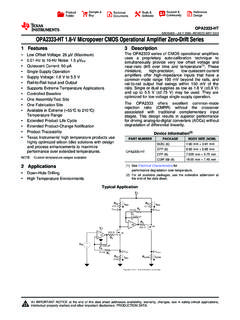
7 Note that the amplifier s rise and fall times may not be exactly equal. So the slew-rate specification of the datasheet is an datasheet slew rate of the OPA2314 amplifier is V/ s and in the system, VPP equals V. While the amplifier is in the linear region, the rail-to-rail output with a power supply is equal to V. Figure 6 shows the tested behavior of the OPA2314 with an output range that goes beyond the linear region of the calculated maximum output voltage of the OPA2314 occurs at approximately kHz. However, in Figure 6, the maximum value with bench data is shown to be approximately 70 kHz. This discrepancy exists because of the mismatches between the amplifier rise and fall times and the responsivity of the amplifier at the peaks and valleys of the sinusoidal input voltage swing. SAR-ADC sampling frequencyThe challenge now is to identify the sampling frequency of the SAR ADC. Given a 1-kHz maximum input signal, it is imperative that the SAR ADC samples the signal more than one cycle per second.

8 Actually, over ten times is pref-erable. This implies that a 10-kHz sampling ADC will work. Additionally, it is important to eliminate signal-path noise when possible. If the SAR ADC is converting at higher frequencies above the corner frequency of the filter , that portion of the noise will not be aliased back into the system. Consequently, a 100-kHz sampling SAR ADC meets the the sampling frequency is 100 kHz, the Nyquist frequency is 50 kHz. At 50 kHz, the frequency response of the low-pass filter is down by approximately 50 dB. This level of attenuation limits the impact on noise going through the development of a DAQ system in the frequency domain can present interesting challenges. A system consisting of a filter and a SAR ADC is usually evaluated with the performance specifications of the DC- and AC-amplifier and the converter. This article, however, evaluated the system s signal path from a frequency important frequency specifications are the signal bandwidth, filter corner frequency , amplifier bandwidth, and converter sampling speed.

9 Even though the signal bandwidth is small, 1 kHz, the required AAF corner frequency should be 10 times higher than the signal band-width in an effort to reduce high- frequency gain errors. Additionally, the converter s sampling frequency is higher than expected in an effort to reduce complications caused by noise Bonnie Baker, Analog filters and specifications swim-ming: Mapping to your ADC, On Board with Bonnie, TI Blog, Nov 5, 2014. 2. Bonnie Baker, Analog Filters and Specification Swimming: Selecting the right bandwidth for your filter , On Board with Bonnie, TI blog, Nov 8, 2013. Related Web sitesTINA-TI WEBENCH to the 6. OPA2314 maximum output voltage6543210 Voltage (V)PP10 k1 M10 M100 kFrequency (Hz)R= 10 kC= 10 pFLL V= VINV= VINV= VINA nalog Applications JournalE2E and TINA-TI are trademarks and WEBENCH is a registered trademark of texas instruments . All other trademarks are the property of their respective Worldwide Technical SupportInternetTI Semiconductor Product Information Center Home E2E Community Home Information CentersAmericas Phone +1(512) 434-1560 Brazil Phone 0800-891-2616 Mexico Phone 0800-670-7544 Fax +1(972) 927-6377 Internet/Email , Middle East, and AfricaPhone European Free Call 00800-ASK- texas (00800 275 83927) International +49 (0) 8161 80 2121 Russian Support +7 (4) 95 98 10 701 Note: The European Free Call (Toll Free) number is not active in all countries.

10 If you have technical difficulty calling the free call number, please use the international number +(49) (0) 8161 80 2045 Internet Email International +81-3-3344-5317 Domestic 0120-81-0036 Internet/Email International Domestic Toll-Free Number Note: Toll-free numbers may not support mobile and IP phones. Australia 1-800-999-084 China 800-820-8682 Hong Kong 800-96-5941 India 000-800-100-8888 Indonesia 001-803-8861-1006 Korea 080-551-2804 Malaysia 1-800-80-3973 New Zealand 0800-446-934 Philippines 1-800-765-7404 Singapore 800-886-1028 Taiwan 0800-006800 Thailand 001-800-886-0010 International +86-21-23073444 Fax +86-21-23073686 Email or Notice: The products and services of texas instruments Incorporated and its subsidiaries described herein are sold subject to TI s standard terms and conditions of sale. Customers are advised to obtain the most current and complete information about TI products and services before placing orders.