dx.doi.org/10.14227/DT110304P25 Statistical Properties of ...

1 Statistical Properties of the dissolution Test of USP. Carlos D. Saccone1,3, Julio Tessore1, Silvino A. Olivera2, and Nora S. Meneces1 email: Abstract The Monte Carlo simulation method is used to study Statistical Properties of the USP dissolution test. Some interesting aspects of immediate release dissolution are presented, including: a. A unified operating curve that allows estimation of the probability of acceptance (Pa) of a lot as a function of its sta- tistical parameters. b. Verification that the Statistical behavior is only slightly affected by the underlying distribution of the individual amounts dissolved. c. The average number of samples required to reach a decision is presented as a function of parameters of the lot. d. The relative influence of the three stages of the test in the probability of acceptance.

2 Introduction the Statistical Properties of the dissolution test. The follow- T. he dissolution test as defined in the United States Phar- ing aspects of immediate release dissolution were studied: macopoeia (1) is used in judging the quality of pharma- ceutical products. dissolution testing is a method for Probability of acceptance of the dissolution test (Pa), e. evaluating physiological availability that depends upon g. probability of passing the test, as a function of the having the drug in a dissolved state. The USP dissolution dissolution population parameters (mean and standard testing involves three stages and the acceptance criteria are deviation expressed as a percentage of label content), defined for each stage as a function of a quantity Q,a Influence of the shape of the population distribution percentage of the label value that is established for each on the probability of acceptance.

3 Drug product in its monograph. Acceptance criteria are Average sample number needed for reaching a deci- shown in Table 1. sion when the test is applied. These acceptance criteria are complex and the behavior Contribution of each stage of the test to the probabili- of the test for samples of varying quality levels is not easily ty of acceptance. predictable from the knowledge of its drug Properties . Pharmaceutical manufacturers are interested in many of Methodology The Monte Carlo simulation method was used to study Table 1. USP Acceptance Criteria Statistical Properties of the dissolution test. Amounts dis- solved, expressed as a percentage of the label value of each unit (tablet, capsules, etc.), were obtained through the use Number of Visual Basic-Excel Statistical routines. In Figure 8, a flow- Stage units Acceptance Criteria chart (similar to the flowchart presented by PHEATT (2) of S1 6 Each unit is not less than Q* +5% the simulation is provided.)

4 More than 100 million dissolu- tion values were generated in order to assure uncertainty S2 6 Average of the 12 (S1+S2) units is values of less than in the probability of acceptance. Q and no uni is less than Q 15% Probability of acceptance, (Pa), and average sample num- S3 12 Average of 24 (S1+S2+S3) units is ber (ASN) were studied in the range of conditions of inter- Q and not more than 2 units are est for the objectives of this study, as shown in Table 2. less than Q 15% and no unit is less than Q 25% Results and Discussion Operating Characteristic Curves *Q is the amount of dissolved active ingredient specified in the individ- ual monograph, expressed as a percentage of the labeled content. The operating characteristic curves of the dissolution test are defined in this paper as Probability of acceptance 1 University of the Republic of Uruguay, Faculty of Engineering, Industrial 3 Corresponding author, Facultad de Ingenier a, Instituto de Ingenier a Production Department, Montevideo, Uruguay Mec nica y Producci n Industrial, Julio Herrera y Reissig 565, Montevideo, 2 University of the Republic of Uruguay, Faculty of Chemistry, Estrella Uruguay Campos Department, Montevideo, Uruguay dissolution Technologies | AUGUST 2004.

5 25. Figure 1. Operating curves for Q = 80, RSD 1 to 10%, Normal distribution. Table 2. Operation Conditions for studying probability of acceptance (Pa) and the average sample number (ASN). Q = 75 Q = 80. Pa ASN Pa ASN. Mean (%) 70 90 50 90 75-95 55 95. RSD (%)* 1 10 1 15 1 10 1 15. Distributions N, LN** N, LN N, LN N, LN. Uncertainty Less than Less than in Pa *RSD: Relative standard deviation Figure 2. Plot of Probability of acceptance of dissolution test as a function of **N, LN: Normal and lognormal distribution. (Mean-Q)/Std. Deviation. Unified curve made by using all the values obtained for Q = 75 and Q = 80 and RSD 1 to 10%. Unified Characteristic Curve As Murphy and Sampson (3) suggested, the curves may be unified representing Pa as a function of a parameter that eliminates the influence of Q and RSD.

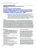
6 The results obtained for Pa as a function of (Mean=Q)/Standard devia- tion are shown in Figure 2. The curve was made by using all the values obtained for Q=75 and Q=80 and RSD 1 to 10%. This curve thus built allows us to easily estimate Pa as a function of dissolution parameters (mean, standard devia- tion). The thickness of the curve indicates the maximum observed variations in the Pa obtained in the simulations performed. These variations observed represent less than approximately in the Pa in all the ranges studied. It can be observed that when the mean value is Figure 3. Plot of the differences between Probabilities of acceptance in disso- standard deviation and less, the Pa is insignificant, and lution test (Normal minus lognormal), assuming Normal and Lognormal dis- when the mean value is Q+ standard deviation and tributions as a function of Mean, Q=75 and RSD 1 to 10%.

7 Solid dots were more, the Pa is almost 1. obtained for RSD between 1 and 8 %, empty dots were obtained for RSD 9. and 10%. Robustness There is no agreement (2) about the shape of the distrib- ution of the dissolved amounts and therefore it was con- sidered important to study how the curves shown above depend on the distribution assumed. Particularly, for nor- mal and lognormal distributions the different Pa have been evaluated. These distributions were chosen for the follow- ing reasons: Normal distribution was considered a good model of the distribution since the amount dissolved by each unit is a function of a large number of variables. Lognormal distribution seems suitable to simulate a (Pa) vs. mean of dissolution values expressed as a percent- physical limit to the amount dissolved due to the age of the label content.

8 They have a characteristic S shape, amount of drug product in the pharmaceutical dosage and are shown in Figure 1. form. If the underlying distribution of amount dis- All the curves, in the range of RSD studied, intercept at a solved is lognormal, a large slope is observed towards mean value equal to Q. This means that at this point, the the right (where the physical limit exists) and a low Probability of acceptance does not depend on RSD and its slope towards the left. value is Pa = For Q=75 a similar behavior is obtained in the shape of the curves and in the intercept value The observed influence on probability of acceptance is (Pa= , mean=Q). shown in Figure 3, and it can be seen that there are not rele- 26 dissolution Technologies | AUGUST 2004. vant differences between normal and lognormal distribu- Figure 4.

9 Ideal curve. Average Sample Number as a function of Mean, Q=75. tions. The probability of passing the test when the data were and RSD=0%. normally distributed differs less than from that of log- normal distribution for population RSD values of 8% or less. As expected, in the range in which the rejections are due to the non-compliance of the requirements on the average value (stages 2 and 3), the central limit theorem assures insensitivity to the distribution shape. When non-compli- ances are due to individual values (clauses Q-25% and Q- 15%), the probability of acceptance is more dependent on the assumed distribution of amount dissolved. This occurs for larger RSDs, 9 and 10%. Average Sample Number The average sample number of units required to arrive at a decision about the test was studied.

10 This number (ASN) is a function of the mean and standard deviation. Ideally, if it is considered that the variability is zero (RSD=0), when the dissolution values increase (Figure 4) it should be expected that: a. Rejection of tests in the first stage if dissolution is less than Q-15% (tested units = 6). b. Three stages are required to reach a decision with dis- Figure 5. Plot of Average Sample Number as a function of Mean, Q=75 and solution values less than Q and more than Q-15% RSD 1 to 15%. (tested units = 24). c. Acceptance in the second stage for dissolution values that are more than Q and less than Q+5% (tested units = 12). d. Acceptance in the first stage for dissolution values that are more than Q +5% (tested units = 6). The curves obtained with variability different to zero, (RSD 1 to 15%) present the four steps described, but they separate from the ideal curve and differences are larger as the RSD increases (Figure 5).