Transcription of Dynamics of the Heavy-Light Spread in the N. American Oil ...
1 Dynamics of the Heavy-Light Spread in the N. American Oil MarketRomain H. Lacombe and John E. ParsonsMIT Energy and Environmental Policy Workshop6-7 December 20072 The Issue North American crude oil marketszLight sweet crude: global light marketzHeavy sour crude: Mexican and Venezuelan oilzNew entrant: heavy products from Canadian oil sands Question: how do heavy and light crude prices relate?zIs there a reliable long run equilibrium? Fixed percent spreads ? Fixed differentials? Other?zWhat about the Dynamics of the market? Short-run responses to shocks? Long-run shifts?3 The Data Focus on three key marker crudes: WTI, LLB and MayazWest Texas Intermediate Blend global light crude marketzLloydminster Blend Canadian heavy crude market (benchmark for Diluted Bitumen from the Athabasca oil sands)zMaya Blend Central and South Am.
2 Heavy crude market Data: weekly prices for the 1998 - 2007zWTI: NYMEX front month contract for delivery at Cushing, OKzLLB: spot contract for delivery at Hardisty, : sold CIF to USGC based on Pemex marked price4 Historical Evolution of Prices0204060801001998w12 000 w12002w12004w12 006 w12008w1Ti me (wee kly )WTI 1st Month NYMEXMaya BlendLloydminster Blend 1998/01:zWTI: : : 2007/11:zWTI: : : rise in pricesVolatility periods:zKatrinazIrakz9/115 Absolute spreads : WTI-Maya and WTI-LLB0102030401998w12 000 w12002w12004w12 006 w12008w1Ti me (wee kly )WTI-LLB DifferentialFitted valuesWTI-Maya DifferentialFitted values0102030401 998 w12 000 w12 002 w12 004 w12 006 w12 008 w1Ti me (wee kly )WTI-LLB DifferentialFitted valuesWT I- Ma ya D if fe ren t ialF it te d v alu esShell shutdownsSuncor shutdownsHurricane Wilma 1998/01:zLLB: : 2007/11:zLLB: : 998 w12 000 w12 002 w12 004 w12 006 w12 008 w1Ti me (wee kly )Fitted valuesFitted valuesMaya/WTI S pr ead (%)LLB/WTI Spread (%)Percent spreads : Maya/WTI and LLB/WTI 1998/01:zLLB: : 2007/11:zLLB: : Keith?
3 Hurricanes Ivan & JeanneHurricane Katrina7 Early Conclusions No simple long run equilibrium relationshipzFixed price differentials exhibit heteroskedasticityzFixed percent spreads are shifting with time Differential shocks impact all marketszGlobal shocks have differentiated local effectszLocal shocks have repercussions on other marketsNeed for thorough time series analysisTime Series Analysis9 Estimating a Model of Price Dynamics Problem in inference on time trended time easy to erroneouslyfind a relationship between 2 series if they are not oil prices went up while steel price went up too: Causality? Correlation?10 Estimating a Model of Price Dynamics Problem in inference on time trended time easy to erroneouslyfind a relationship between 2 series One solution is to first detrend the series, , by taking first differenceszthis works sometimes, but the underlying problem is sometimes more subtle and undermines the validity of this simple for oil and steel -- if energy prices impact steel price, the following structure may prevail.
4 ZIn that case, differencing ignores long run equilibrium between the variables due to the shared stochastic trend OilEnergyOilSteelEnergySteelPPPP+=+=11 Estimating a Model of Price Dynamics Problem in inference on time trended time easy to erroneouslyfind a relationship between 2 series One solution is to first detrend the series, , by taking first differenceszThis works sometimes, but the underlying problem is sometimes more subtle and undermines the validity of this simple solution Resolution: cointegration analysiszSearch for the cointegration a more robust search through a broader universe of possible stationary linear combinations of the non-stationary variableszIf variables reversal to a long run equilibriumPPOilSteel 12 Traditional Diagnostics Standard VAR(p) model:Test lag order p Standard estimation method: VAR(p) modelzWorks for stationary variableszStandard form assumes no contemporaneous effect of variables on each other zStructural form (informed by standard form) can allow contemporaneous effects tpiititPAP+ == 1 Structural VAR(p) model.
5 TpiitittPABPP+ +== 1 Structural assumptions13 Traditional Diagnostics Estimation method for non-stationary variables: VECM modelzFirst differences of VAR(p) model in standard formzImplies linear combination of lagged price levels is stationaryzHence need to choose a constraint on rank Johansen testVECM(p,r) model: ttpiititPPP++ = = 111 Test lag order pJohansen test for rank rStationary linear combinationCECM(p,r) model: ttpiititPPP++ = = 110 Structural assumptions14 Overview of the Path for EstimationStandard VAR(p) model:Test lag order p tpiititPAP+ == 1 Structural VAR(p) model: tpiitittPABPP+ +== 1 VECM(p,r) model: ttpiititPPP++ = = 111 Test lag order pJohansen test for rank rCECM(p,r) model: ttpiititPPP++ = = 110 Unit root test Stationary VAR Integrated VECM15 Traditional Diagnostics: Unit Root Tests Philipps-Perron unit root testzNull hypothesis: price variables exhibit a unit rootzFirst differences are found stationary by the same test Conclusion: price variables are integrated of order 1 they behave like random walks need for co-integration analysis!
6 ZVECM to reveal long run equilibrium and link with short run dynamicszCECM if specific structure is for null hypothesislog Mayalog LLBlog WTIV ariableVariables exhibit unit roots16 Bottom-line: Cointegration of Crude Prices Part #1. Long-run equilibrium relationship: co-integration framework between WTI, Maya and LLBzDiagnostics: lag order 4, rank 2zReveals long run equilibrium Part #2. Linking short-run to long-run Dynamics : Vector Error Correction Model (VECM)zHighlights relationship between long run equilibrium and short rum dynamicszReveals underlying asymmetry between WTI and the other variables Part #3. Imposing structure on short run Dynamics : Conditional Error Correction Model (CECM)zWTI is assumed exogenouszWe study its contemporaneous and long-run effect on heavy crudes prices17 Part #1 Bottom Line: Long-run Equilibrium Long run equilibrium between LLB and WTI:zlog LLB = (- ) + ( ) log WTI Predicted equilibrium in price levels:02040608010030405060708090100W TI priceLLB priceLLBWTI@$30: 51% Spread to WTI@$100: 59% Spread to WTI18 Part #1 Bottom Line: Long-run Equilibrium (cont.)
7 Historical priceszActual and predicted priceszDeparture from equilibrium0204060801 998 w12000w12002w12 004 w12006w12008w1Ti me (wee kly )Lloydminster BlendLLB (LR)-10-505101 998 w12000w12002w12 004 w12006w12008w1w_ti meDi seq u i l ib ri u m ( L LB t o LL B L R)Ref er en ce1902040608010030405060708090100 WTI priceLLB priceMayaWTIPart #1 Bottom Line: Long-run Equilibrium (cont.) Long run equilibrium between Maya and WTI:zlog Maya = (- .2773277) + ( ) log WTI Predicted equilibrium in price levels:@$30: 82% Spread to WTI@$100: 85% Spread to WTI20 Part #1 Bottom Line: Long-run Equilibrium (cont.) Historical Maya priceszActual and predicted prices0204060801998w12000w12002w12004w12 006w12008w1Ti me (wee kly )Ma ya B len dMa ya ( L R)zDeparture from equilibrium-10-5051 998 w12000w12002w12 004 w12006w12008w1w_ti meDi seq u i li b riu m ( Ma ya t o M aya LR )R ef er en ce21 Part #2 Bottom Line: Short-run Dynamics Shocks to WTI zAffect LLB and Maya in the short runzImpose a strong drag to equilibrium on both heavy crudes Shocks to LLB and MayazAffect WTI in the short runzBut drag to equilibrium is not significant.
8 WTI is weakly exogenous Shocks to LLB zAffect Maya in the short runzImbalance between LLB and WTI affects Maya in the long run Shocks to Maya zAffect LLB in the short runzImbalance between Maya and WTI does not affect LLB22 Part #2 Bottom Line: Short-run Dynamics (cont.) Shocks to WTI cause short run shocks to Maya and LLB Once WTI is stabilized, shocks are persistent and impact long run prices of Maya & LLB zConvergence to long-run equilibrium takes over after 9 10 15 20 25 30 35 40 45 50 Time (weeks)Shock to log variablesDeltaWTID eltaMayaDeltaLLB23 Part #2 Bottom Line: Short-run Dynamics (cont.)303540455055606570051015202530354 045 WTILR MayaLR LLBMayaLLBWTI price shockLong term persistence: of initial shockzLong run pass-through to Maya: 75% of persistent shockzLong run pass through to LLB: 54% of persistent shockInitial adaptation of pricesLong run convergence to equilibrium24 Part #2 Bottom Line: Short-run Dynamics (cont.)
9 Shocks to LLB cause short term shocks to other variables Once other variables have stabilized, LLB has limited further impact on long-run priceszConvergence to long-run equilibrium takes over after 5 10 15 20 25 30 35 40 45 50 Time (weeks)Shock to log variablesDeltaWTID eltaMayaDeltaLLB25zLong run pass-through to WTI: 43% of initial shockzLong run pass through to Maya: 42% of initial shockPart #2 Bottom Line: Short-run Dynamics (cont.)303540455055606505101520253035404 5 WTILR MayaLR LLBMayaLLBLLB price shockInitial adaptation of pricesLong run convergence to equilibriumLong term persistence: of initial shock26 Part #2 Bottom Line: Short-run Dynamics (cont.)
10 Shocks to Maya cause short term shocks to other variables Once other variables have stabilized, Maya has no further impact on long-run priceszConvergence to long-run equilibrium takes over after 6 10 15 20 25 30 35 40 45 50 Time (weeks)Shock to log variablesDeltaWTID eltaMayaDeltaLLB27 Part #2 Bottom Line: Short-run Dynamics (cont.)303540455055606505101520