Transcription of ECON4150 - Introductory Econometrics Lecture 4: Linear ...
1 ECON4150 - Introductory Econometrics Lecture 4: Linear regression with One Regressor Monique de Haan Stock and Watson Chapter 4. 2. Lecture outline The OLS estimators The effect of class size on test scores The Least Squares Assumptions E (ui |Xi ) = 0. (Xi , Yi ) are Large outliers are unlikely Properties of the OLS estimators unbiasedness consistency large sample distribution The compulsory term paper 3. The OLS estimators Question of interest: What is the effect of a change in Xi on Yi ? Yi = 0 + 1 Xi + ui Last week we derived the OLS estimators of 0 and 1 : c0 = Y b1 X.. 1. Pn n 1 i=1 (Xi X )(Yi Y ) sxy . c1 = 1. Pn = sx2. , n 1 i=1 (Xi X )(Xi X ).
2 4. OLS estimates: The effect of class size on test scores Friday January 13 14:48:31 2017 Page 1. Question of interest: What is the effect of a change in class size on test ___ ____ ____ ____ ____(R). scores? /__ / ____/ / ____/. ___/ / /___/ / /___/. TestScorei = 0 + 1 ClassSize i + u i Statistics/Data analysis 1 . regress test_score class_size, robust Linear regression Number of obs = 420. F(1, 418) = Prob > F = R-squared = Root MSE = Robust test_score Coef. Std. Err. t P>|t| [95% Conf. Interval]. class_size .5194892 _cons \ i = ClassSizei TestScore 5. The Least Squares assumptions Yi = 0 + 1 Xi + ui Under what assumptions does the method of ordinary least squares provide appropriate estimators of 0 and 0 ?
3 Under what assumptions does the method of ordinary least squares provide an appropriate estimator of the effect of class size on test scores? The Least Squares assumptions: Assumption 1: The conditional mean of ui given Xi is zero E (ui |Xi ) = 0. Assumption 2: (Yi , Xi ) for i = 1, .., n are independently and identically distributed ( ). Assumption 3: Large outliers are unlikely . 0 < E Xi4 < & 0 < E Yi4 < . 6. The Least Squares assumptions: Assumption 1. E (ui |Xi ) = 0. The first OLS assumption states that: All other factors that affect the dependent variable Yi (contained in ui ) are unrelated to Xi in the sense that, given a value of Xi , the mean of these other factors equals zero.
4 In the class size example: All the other factors affecting test scores should be unrelated to class size in the sense that, given a value of class size, the mean of these other factors equals zero. 7. The Least Squares assumptions: Assumption 1. The first OLS assumption can also be written as: E (Yi |Xi ) = E ( 0 + 1 Xi + ui |Xi ). Expectation rules = 0 + 1 E (Xi |Xi ) + E (ui |Xi ). ASS#1 : E (ui |Xi ) = 0. = 0 + 1 Xi 8. The Least Squares assumptions: Assumption 1. E (Yi |Xi ) = 0 + 1. 9. The Least Squares assumptions: Assumption 1. Example of a violation of assumption 1: Suppose that districts which wealthy inhabitants have small classes and good teachers these districts have a lot of money which they can use to hire more and better teachers districts with poor inhabitants have large classes and bad teachers.
5 These districts have little money and can hire only few and not very good teachers In this case class size is related to teacher quality. Since teacher quality likely affects test scores it is contained in ui . This implies a violation of assumption 1: E (ui |ClassSizei = small) 6= E (ui |ClassSizei = large) 6= 0. 10. The Least Squares assumptions: Assumption 2. (Yi , Xi ) for i = 1, .., n are If the sample is drawn by simple random sampling assumption 2 will hold Example: What is effect of mother's education (Xi ) on child's education (Yi ). Example of simple random sampling: randomly draw sample of mother's with information on her education and the education of one randomly selected child (Yi , Xi ) for i = 1.
6 , n are Example of a violation of simple random sampling randomly draw sample of mothers with information on her education and the education of all of her children. (Yi , Xi ) for i = 1, .., n are NOT Observations on children from the same mother are not independent! 11. The Least Squares assumptions: Assumption 3. Large outliers are unlikely . 0 < E Xi4 < & 0 < E Yi4 < . Outliers are observations that have values far outside the usual range of the data Large outliers can make OLS regression results misleading Another way to state assumption is that X and Y have finite kurtosis. Assumption is necessary to justify the large sample approximation to the sampling distribution of the OLS estimators 12.
7 The Least Squares assumptions: Assumption 3. 13. Use of the Least Squares assumptions Yi = 0 + 1 Xi + ui Assumption 1: E (ui |Xi ) = 0. Assumption 2: (Yi , Xi ) for i = 1, .., n are Assumption 3: Large outliers are unlikely If the 3 least squares assumptions hold the OLS estimators b0 and b1. Are unbiased estimators of 0 and 1. Are consistent estimators of 0 and 1. Have a jointly normal sampling distribution 14. Properties of the OLS estimator: unbiasedness Yi = 0 + 1 Xi + ui Y = 0 + 1 Xi + u Pn . (Xi X )(Yi Y ). h i i=1. E b1 =E Pn i=1 (Xi X )(Xi X ). substitute for Yi , Y. Pn . i=1 (Xi X )( 0 + 1 Xi +ui ( 0 + 1 X +u)). =E Pn i=1 (Xi X )(Xi X ).
8 Rewrite ( 0 drops out). Pn . i=1 (Xi X )( 1 (Xi X )+(ui u)). =E Pn i=1 (Xi X )(Xi X ). rewrite & use expectation rules Pn Pn . 1 i=1 (Xi X )(Xi X ) i=1 (Xi X )(ui u). = E Pn X X X X + E Pn X X X X. i=1 ( i )( i ) i=1 ( i )( i ). 15. Properties of the OLS estimator: unbiasedness .. 1 ni=1 (Xi X )(Xi X ). Pn (Xi X )(ui u). h i P. i=1. E b1 =E Pn +E Pn i=1 ( i X X )(Xi X ) i=1 ( i X X )(Xi X ). take 1 out of 1st expectation Algebra trick Pn . (Xi X )ui = 1 + E Pn i=1. i=1 ( i X X )(Xi X ). Law of iterated expectations Pn . (X X )E[ui |Xi ]. = 1 + E Pni=1 X i X X X. i=1 ( i )( i ). h i E b1 = 1 if E [ui |Xi ] = 0. 16. Algebra trick Pn Pn Pn Pn Pn i=1 Xi X (ui u) = i=1 Xi ui i=1 Xi u i=1 X ui + i=1 Xu Pn 1.
9 Pn Pn = i=1 Xi ui n n i=1 Xi u i=1 X ui + nX u Pn Xi ui nX u + ni=1 X ui +nX u P. = i=1. = ni=1 Xi ui ni=1 X ui P P. P . = ni=1 Xi X ui 17. Consistency p b1 1. Consistency: or plim b1 = 1. Pn . i=1 (Xi X )(Yi Y ). Plim b1 = plim Pn i=1 (Xi X )(Xi X ). 1 Pn Plim n 1 i=1 (Xi X )(Yi Y ) sXY. = 1 Pn = 2. i=1 ( i Plim n 1 X X )(Xi X ) sX. law of large numbers OLS assumptions 2 and 3. Cov (Xi ,Yi ). = Var (Xi ). substitute for Yi Cov (Xi , 0 + 1 Xi +ui ). = Var (Xi ). see Key Concept 1 Var (Xi )+Cov (Xi ,ui ). = Var (Xi ). 18. Consistency 1 Var (Xi )+Cov (Xi ,ui ). Plim b1 = Var (Xi ). = 1 Var (Xi ). Var (X ). + Cov (Xi ,ui ). Var (Xi ). i substitute covariance expression E[(Xi x )(ui u )].
10 = 1 + Var (Xi ). algebra trick E[(Xi x )ui ]. = 1 + Var (Xi ). Law of iterated expectations E[(Xi x )E[ui |Xi ]]. = 1 + Var (Xi ). so Plim b1 = 1 if E [ui |Xi ] = 0. 19. Unbiasedness vs Consistency Unbiasedness & consistency both rely on E [ui |Xi ] = 0. h i Unbiasedness implies that E b1 = 1 for a given sample size n Consistency implies that the sampling distribution becomes more and more tightly distributed around 1 if the sample size n becomes larger and larger. 20. Consistency: A simulation example Lets create a data set with 100 observations Xi N(0, 1). ui N(0, 1). We define Y to depend on X as: Yi = 1 + 2Xi + ui Thursday January 19 12:00:40 2017 Page 1.