Transcription of EE363 homework 4 solutions - Stanford University
1 EE363 Prof. S. BoydEE363 homework 4 an unknown constant from repeated wish to estimatex N(0,1) from measurementsyi=x+vi,i= 1, .. , N, whereviare IIDN(0, 2),uncorrelated withx. Find an explicit expression for the MMSE estimator x, and theMMSE :We write the relationship between the measurementsyifori= 1, .. , N, andxinmatrix form as = x+ or more compactly asy=Ax+vwherey= (y1, .. , yN),A=1andv= (v1, .. , vN).Now we can use the formulas for the MMSE estimator in the linear measurements caseto obtain x= x+ xAT(A xAT+ v) 1(y y)=1T(11T+I 2v) 1y= (1T1+ 2v) 11Ty=1 TyN+ the error covariance we have est= x xAT(A xAT+ v) 1A x= 1 1T(11T+I 2v) 11= 1 (1T1+ 2v) 11T1= 2vN+ that asN (we perform many measurements), est 0, and as (verylarge noise), est 1 = x( , our prior covariance ofx).
2 Both of these limitingcases make intuitive sense. In the first case by making many measurements we are ableto estimatexexactly, and in the second case with very large noise, the measurementsdo not help in estimatingxand we cannot improve the a priori covariance error variance and correlation (x, y) R2is Gaussian,and let xdenote the MMSE estimate ofxgiveny, and xdenote the expected value ofx. We define the relative mean square estimator error as =E( x x)2/E( x x) that can be expressed as a function of , the correlation coefficient your answer make sense?
3 Solution:Sincex, y Rwe haveE( x x)2=Tr est= x xy 1y Txy,where x= 2x, xy= xy, y= we haveE( x x)2= 2x 2xy course we haveE( x x)2= 2x, so =E( x x)2E( x x)2= ( 2x 2xy 2y)/ 2x= 1 xy x y!2= 1 answer makes perfect sense. Whenxandyhave strong (positive or negative)correlation,| |is close to one, and therefore is close to zero, which mean that therelative minimum mean square estimation error is small. On the other hand, ifxandyare almost uncorrelated, ,| |is small, we find that 1, which mean that theminimum mean square error is close to the prior variance ofx.
4 In other words, whenxandyare highly correlated, we can estimatexfromyaccurately, while whenxandyare uncorrelated, the measurementydoes not help at all in predictor and scalar time seriesy(0), y(1), ..is modeled asy(t) =a0w(t) +a1w(t 1) + +aNw(t N),wherew( N), w( N+ 1), ..are IIDN(0,1). The coefficientsa0, .. , aNare known.(a)Predicting next value from current the MMSE predictor ofy(t+ 1)based ony(t). (Note: we really mean based on justy(t), and not based ony(t), y(t 1), ..) Your answer should be as explicit as possible.(b)MMSE the MMSE predictor ofy(t) (fort >1) based (only)ony(t 1) andy(t+ 1) (fort 1).
5 Your answer should be as explicit as :(a)Predicting next value from current ll use the general expression for the MMSE estimator: y(t+ 1) = y(t+ 1) + y(t+1)y(t) 1y(t)(y(t) y(t))= y(t+1)y(t) 1y(t)y(t)2(since thew s are all zero mean, which implies they s are all zero mean). Nowwe will find y(t+1)y(t)and y(t): y(t)=E(a0w(t) +a1w(t 1) + +aNw(t N))2=NXi=0a2iusing the fact thatEw(t)w(s) = t s. Similarly we have y(t+1)y(t)=E(a0w(t+ 1) +a1w(t) + +aNw(t+ 1 N))(a0w(t) + +aNw(t N))=N 1Xi=0ai+ the MMSE estimator is: y(t+ 1) =PN 1i=0ai+1aiPNi=0a2iy(t).
6 This expression makes sense: you just multiply what you justobserved (y(t)) bya constant to predicty(t+ 1). (The constant, by the way, is between zero andone.)(b)MMSE (t) = [y(t+ 1)y(t 1)]T. We want to find y(t) =E(y(t)|z(t)). We first find the required covariance matrices: y(t)z(t)=Ey(t)[y(t+ 1)Ty(t 1)T] ="N 1Xi=0ai+1aiN 1Xi=0ai+1ai#and z(t)=E[y(t+ 1)y(t 1)]T[y(t+ 1)y(t 1)] ="PNi=0a2iPN 2i=0ai+2aiPN 2i=0ai+2aiPNi=0a2i#Therefore the MMSE interpolator is y(t) ="N 1Xi=0ai+1aiN 1Xi=0ai+1ai#"PNi=0a2iPN 2i=0ai+2aiPN 2i=0ai+2aiPNi=0a2i# 1"y(t+ 1)y(t 1)#We find the inverse of the 2 2 matrix z(t)and multiply out to obtain the finalresult: y(t) =PN 1i=0ai+1aiPNi=0a2i+PN 2i=0ai+2ai[y(t+ 1) +y(t 1)].
7 So the MMSE interpolator takes the average of the two observationsy(t 1) andy(t+ 1), and multiplies it by a initial subpopulations from total growth sample that con-tains three types of bacteria (called A, B, and C) is cultured, and the total bacteriapopulation is measured every hour. The bacteria populations grow, independently ofeach other, exponentially with different growth rates: A grows 2% per hour, B grows5% per hour, and C grows 10% per hour. The goal is to estimate the initial bacteriapopulations based on the measurements of total (t) denote the population of bacteria A afterthours (say, measured in grams),fort= 0,1.
8 , and similarly forxB(t) andxC(t), so thatxA(t+ 1) = (t), xB(t+ 1) = (t), xC(t+ 1) = (t).The total population measurements arey(t) =xA(t) +xB(t) +xC(t) +v(t), wherev(t)are IID,N(0, ). (Thus the total population is measured with a standard deviationof ).The prior information is thatxA(0), xB(0), xC(0) (which are what we want to estimate)are IIDN(5,2). (Obviously the Gaussian model is not completely accurate since itallows the initial populations to be negative with some small probability, but we llignore that.)How long will it be (in hours) before we can estimatexA(0) with a mean square errorless than How long forxB(0)?
9 How long forxC(0)?Solution:Afterthours we have madet+ 1 measurements: y(0)..y(t) =F(t) xA(0)xB(0)xC(0) + v(0)..v(t) , F(t) = .The covariance of the noise vector [v(0) v(N)]tis The prior covariance of[xA(0)xB(0)xC(0)]tis the covariance of the estimation error is est(t) = (F(t)T( ) 1F(t) + (2I) 1) 1= (4F(t)TF(t) + ) mean-square error in estimatingxA(0) is given by the (1,1) entry of est; forBandCit is given by the other diagonal elements. So what we need to do is to find howlargethas to be before the diagonal elements of est(t) become less than Thiscan be done by plotting, or any other method.
10 The plot below shows the mean-squareerror in estimatingxA(0),xB(0), andxC(0), as a function oft. The shape of the plotmakes good intuitive sense, if you think about it long most rapidlyso it is not surprising that we can estimatexA(0) accurately more quickly than the4other two. (If anyone can think of an intuitive explanation of the flat part betweent= 10 andt= 20 in the estimation error forxA(0), I d like to hear it!)The solution is: 79 hours forxA(0), 60 hours forxB(0), and 32 hours forxC(0). xA(0) xA(0)k2Ek xB(0) xB(0)k2Ek xC(0) xC(0)k2A=diag([ ]); C=[1 1 1];sigma= ; S_x=2*eye(3);;AA=eye(3); O=[]; a=[]; b=[]; c=[];t=0;while 1O=[O;C*AA];AA=A*AA;S_est=inv( *eye(3)+O *O/sigma^2);a=[a;S_est(1,1)];b=[b;S_est( 2,2)];c=[c;S_est(3,3)];if max([a(t+1),b(t+1),c(t+1)]) <= +1;end% plot MMSE estimation errorsclgsubplot(3,1,1)5plot(linspace(0, t,t+1),a); grid on; xlabel( t );ylabel( A )subplot(3,1,2)plot(linspace(0,t,t+1),b) ; grid on; xlabel( t );ylabel( B )subplot(3,1,3)plot(linspace(0,t,t+1),c) ; grid on; xlabel( t ).