Transcription of EGN1006 - Mathcad fundamentals and functions III
1 Mathcad fundamentals and functions Session IIIEGN 1006 introduction to EngineeringMATHCADData Analysis and Statistical AnalysisAnalysisStatistical FunctionsMATHCAD offers the capability to perform statistical analysis by a number of built-in functions that can be applied directly to the data contained in single or multi-dimensional arraysdimensional arrays mean(A)Mean or Average stdev(A)Standard Deviation var(A)VarianceEnter the followingCreate a matrix A with 11 rows and 1 column. Enter the following values as shown then type:shown then type:mean(A)=stdev(A)=var(A)=Interpolati on FunctionsMATHCAD is capable of automatically interpolating data using several degrees of approximation linterp(Vx,Vy,p)Linear Interpolationlspline(V,V)Linear Spline lspline(Vx,Vy)Linear Spline pspline(Vx,Vy)Parabolic Spline cspline(Vx,Vy)Cubic Spline interp(Vs,Vx, ) General Interpolation from spline output corr(Vx1,Vx2)correlates two arrays for residualsWhat is a spline?
2 The linear spline represents a set of line segments between the between the two adjacent data pointsEnter the followingCreate an 11r,1c Matrix called time and enter the values an 11r,1c Matrix called T and enter the values shownDo the followingCreate an X-Y plot with time on the x-axis. Change the graph so that the data is represented by points and symbolic o s (Double click on graph)symbolic o s (Double click on graph)Question:What would the temp be at seconds?EnterLinterp(time,T, )=Higher order interpolationThe value of the linear interpolation is just a general trend value and may not be very :Vs:=cspline(time,T)Vs= ( just to take a peek at it, then erase it)sEnter: (General interpolation)interp(Vs,time,T, )=The Algorithms to calculate this value is COMPLICATED! But it is a built in Mathcad function!
3 Curve Fitting FunctionsMATHCAD includes several functions that produce the coefficients for several curve models. intercept(Vx,Vy)linear y-intersection intercept(Vx,Vy)linear y-intersection slope(Vx,Vy)linear slope linfit(Vx,Vy,f)generalized regressionProduces as many coefficients as required by the dimensions of the function f Enter the followingOur time/temp graph may look straight but we cannot assume it :=intercept(time,T)b:=intercept(time,T)b =m:=slope(time,T)m=Do the followingLet s say we want to see the line of best fit! Copy and Paste the graph underneath all current the following ABOVE the pasted graph:Note: The T(linear) uses BOTH a text subscript AND an index subscript). Also, notice that we are using the equation of a line y=mx+bDo the followingClick on the T on the graph then hit the comma key on the keyboard.
4 This keyboard. This will create another entry box. Enter in T(linear) then hit enter. You should see:A general regressionFirst we must define a function f . Create and define a function f(x) as a 3x1 matrix as shown. This matrix represents the equation of a parabola a+bx+cx2. Then define a using linfit commandEnter:a=These are the COEFFICIENTS in the parabola equationEnter the followingBegin by defining a RANGE variable I . Then define T(parab) indexed by i as shown below. Remember that TIME is on the x-axis so it replaces x in the equation. Each a is INDEXED by a place equation. Each a is INDEXED by a place in the matrix, so make sure you use appropriate index keystrokesDo the followingClick on the T on the graph and once again hit the comma key to insert a NEW line insert a NEW line on the graph, with this one being parabolic in nature.
5 You should see:How CLOSE is the data?We now want to compare how the T(linear) and the T(parab) fit with the original data T .Enter this below the graphEnter this below the graphcorr(Tlinear,T)=corr(Tparab,T)=You can easily see which one is a better fit as we desire to get a value close to ONE!Special Regression FunctionsMATHCAD can also do the following: expfit(Vx,Vy,Vg) lgsfit(Vx,Vy,Vg)beaxycaexybx+=+= 1)()( lgsfit(Vx,Vy,Vg) logfit(Vx,Vy,Vg) pwrfit(Vx,Vy,Vg) sinfit(Vx,Vy,Vg)Vgis an optional array of guessed coefficientscbxaxycaxxycxaxybebbx++=+=+= + )sin()()()ln()(1 Enter the followingFirst we will define a special array of guessed coefficients. Define Vgas a 3x1 matrix Vgas a 3x1 matrix as shown. The define a then enter a=to see the REAL coefficients. You should see:Try this!
6 Using what you have already done,REPEAT this entire process and do an EXPONENTIAL fit. Add the exponential curve on a second exponential curve on a second pasted graph and do a correlation between Texpand TDO NOT LOOK AT THE NEXT SLIDE UNTIL TOLD!YOU SHOULD SEEYou should seeComplete the following assignment