Transcription of Electrochemical Impedance Spectroscopy (EIS) …
1 Autolab Application Note EIS05 Electrochemical Impedance Spectroscopy (EIS) part 5 Parameter estimation Keywords Electrochemical Impedance Spectroscopy ; frequency response analysis; Nyquist and Bode presentations; data fitting; equivalent circuit; parameter estimation Summary In the previous application note on equivalent circuit models, an overview of the different circuit elements that are used to build an equivalent circuit model was given. It was shown that these circuit elements provide the building blocks for more complex models. After identifying a suitable model for the system under investigation, the next step in the data analysis is estimation of the model parameters. This is done by the non-linear regression of the model to the data.
2 Most Impedance systems come with a data-fitting program. Although these programs can be used as a black box, care must be taken to avoid problems. Weighting the data The fitting of a model to data is the minimization of the objective function, J, using a non-linear regression routine: = , , , + , , , where: , , , are the real and imaginary data , , , are the real and imaginary model , , , are the real and imaginary weights There are several different weighting strategies that are possible. The three most common strategies are described in this section. No weighting In Impedance Spectroscopy the value of low frequency data points is usually much larger than that of the high frequency data points (sometimes by several orders of magnitude).
3 , = , = 1 When no weighting is used then the low frequency points would have higher weight than the high frequency points. This introduces a bias and can give large errors in parameter estimation . Therefore, this weighting should not be used. Proportional weighting Usually at high and low frequencies the imaginary part of the data goes to zero. , = , , = , In that case proportional weighting can cause numerical problems because of division by zero. Therefore, this weighting should not be used. Modulus weighting Weighting the data by the absolute value of Impedance is the most recommended weighting strategy and is the default weighting in the AUTOLAB software. , = , =| | Initial Guess The models in Impedance Spectroscopy are highly non-linear in parameter space, which implies that the objective function can have several local minima.
4 An initial guess of the parameters is required to begin the regression procedure. A poor choice of the initial guess can result in the procedure terminating at a local minimum with, for example, wrong estimates for the model parameters. A good initial guess requires some experience. An examination of asymptotes and inflexion points in the Nyquist and Bode diagrams can give some clues for making a good initial guess. Autolab Application Note EIS05 Electrochemical Impedance Spectroscopy (EIS) part 5 Parameter estimation Page 2 of 2 In the following figure the errors that can be introduced due to bad initial guess are illustrated. The circles represent the experimental data. The solid line is the result of fit to the data using a good initial guess, and the dotted line represents the result with a poor initial guess.
5 One can see that a poor initial guess can result in poor fit of the model to the data. Non-uniqueness of circuit models The Impedance spectrum, shown in the following figure, shows two clearly defined semi circles. An equivalent circuit that consists of two RC time constants can model this spectrum. The two RC time constants can be produced by combining the resistances and capacitances in three different ways resulting in three equivalent circuits shown in the following figure. All three circuits when fitted to the data would give an identical fit, with only the circuit parameters being different. In this case, there is no unique equivalent circuit that describes the spectrum. One cannot assume that an equivalent circuit that produces a good fit to a data set represents an accurate physical model of the cell.
6 One needs prior knowledge or complementary experiments to determine the appropriate model for the data. This is one of the limitations of Impedance Spectroscopy . Equivalent Circuit Models with Two Time Constants The three equivalent circuits shown above are mathematically identical. Date 1 July 2011 Bad fitBad fitBad fitBad fit Good fitGood fitGood fitGood fit