Transcription of Estimation and Confidence Intervals
1 Estimation and Confidence IntervalsFall 2001 Professor Paul GlassermanB6014: Managerial Statistics403 Uris HallProperties of Point Estimates1. We have already encountered twopoint estimators:thesamplemeanXis an estimatorof the population mean , and the sample proportion pis an estimator of the populationproportionp. These are called point estimates in contrast tointerval estimate is a single number (suc hasXor p) whereas an interval estimate gives arangelikely to contain the true value of the unknown What makes one estimator better than another? Is there some sense in whichXand pare the best possible estimates of andp, given the available data?
2 We briefly discussthe relevant considerations in addressing these There are two distinct considerations to keep in mind in evaluating an estimator:biasand variability. Variability is measured by the standard error of the estimator, and wehave encountered this already a couple of times. We have not explicitly discussed biaspreviously, so we focus on it In everyday usage,biashas many meanings, but in statistics it has just one: the bias of anestimator is the difference between its expected value and the quantity being estimated:Bias(estimator) =E[estimator] quantity being estimator is calledunbiasedif this difference is zero.
3 , ifE[estimator] = quantity being The intuitive content of this is that an unbiased estimator is one that does not systemat-ically overestimate or underestimate the target We have already met two unbiased estimators: the sample meanXis an unbiased es-timator of the population mean becauseE[X]= ; the sample proportion pis anunbiased estimator of the population proportionpbecauseE[ p]=p. Eac hof t hese esti-mators is correct on average, in the sense that neither systematically overestimates We have discussed Estimation of a population mean but not Estimation of a popula-tion variance 2from a random sampleX1.
4 ,Xnusing thesamplevariances2=1n 1n i=1(Xi X)2.(1)It is a (non-obvious) mathematical fact thatE[s2]= 2; , the sample variance isunbiased. That s why we divide byn 1; if we divided byn, we would get a slightlysmaller estimate and indeed one that is biased low. Notice, however, that even if wedivided byn, the bias would vanish asnbecomes large because (n 1)/napproaches Thesample standard deviations= 1n 1n i=1(Xi X)2is not an unbiased estimator of the population standard deviation .Itisbiasedlow,becauseE[s]< (this isn t obvious, but it s true). However, the bias vanishes as thesample size increases, so we use this estimator all the The preceeding example shows that a biased estimator is not necessarily a bad estimator,so long as the bias is small and disappears as the sample size Intervals for the Population Mean1.
5 We have seen that the sample meanXis an unbiased estimator of the population mean . This means thatXis accurate, on average; but of course for any paricular data setX1,..,Xn,thesamplemeanmaybehigherorlo werthanthetruevalue . The purposeof aconfidence intervalis to supplement the point estimateXwit hinformation aboutthe uncertainty in this A confidence interval for takes the form X , with the range chosen so that thereis, , a 95% probability that the error X is less than ; ,P( <X < ) =. know thatX is approximately normal wit hmean 0 and standard deviation / , to capture the middle 95% of the distribution we should set = can now say that we are 95% confident that the true mean lies in the interval (X n,X+ n).
6 This is a95% confidence intervalfor .3. In deriving this interval , we assumed thatXis approximately normalN( , 2/n). Thisis valid if the underlying population (from whichX1,..,Xnare drawn) is normal or elseif the sample size is sufficiently large (sayn 30).4. Example: Apple Tree Supermarkets is considering opening a new store at a certain loca-tion, but wants to know if average weekly sales will reac h$250,000. Apple Tree estimatesweekly gross sales at nearby stores by sending field workers to collect observations. Thefield workers collect 40 samples and arrive at a sample mean of $263, thestandard deviation of these samples is $42,000.
7 Find a 90% confidence interval for .If we ask for a 90% confidence interval , we should use instead of as the multi-plier. This is interval is thus given by(263590 (42000/ 40),263590 + (42000/ 40))which works out to be 263,590 10,924. Since $250,000 falls outside the confidenceinterval, Apple Tree can be reasonably confident that their minimum cut-off is Statistical interpretation of a confidence interval : Suppose we repeated this samplingexperiment 100 times; that is, we collected 100 different sets of data, each set consistingof 40 observations. Suppose that we computed a confidence interval based on each of the100 data sets.
8 On average, we would expect 90 of the confidence Intervals to include thetrue mean ; we would expect that 10 would not. The figure 90 comes from the fact thatwe chose a 90% confidence More generally, we can choose whateverconfidence levelwe want. The convention is tospecify the confidence level as 1 ,where is typically , or These three values correspond to confidence levels 90%, 95% and 99%. ( is the Greek letter alpha.)7. Definition: For any between 0 and 1, we definez to be the point on thez-axis suchthat the area to the right ofz under the standard normal curve is ; ,P(Z>z )=.
9 See Figure Examples: If =.05, thenz = ; if =.025, thez = ; if =.01, thenz = These values are found by looking up 1 We can now generalize our earlier 95% confidence interval to any level of confidence 1 :X z /2 4 3 2 z 4 3 2 /2z /2 z /2 /2 Figure 1: The area to the right ofz is . For example, The area outside z /2is /2+ /2= . For example, so the area to the right of is , the areato the left of is also , and the area outside is . Whyz /2, rather thanz ? We want to make sure that the total area outside the intervalis . This means that /2 should be to the left of the interval and /2 should be to theright.
10 In the special case of a 90% confidence interval , = , so /2= , Here is a table of commonly used confidence levels and their multipliers:Confidence Level /2z /290% Variance, Large Sample1. The expression given above for a (1 ) confidence interval assumes that we know 2,thepopulation variance. In practice, if we don t know we generally don t know , this formula is not quite ready for immediate When we don t know , we replace it wit han estimate. In equation (1) we have anestimate for the population variance. We get an estimate of the population standarddeviation by taking the square root:s= 1n 1n i=1(Xi X) is thesample standard deviation.