Transcription of Excel - last cell in a range
1 Finding the last cell in an Excel range Using built in Excel functions to locate the last cell containing data in a range of cells . There are all sorts of times in Excel when you will need to find the last cell in a range . For instance, in using a dynamic range name, it is vital to be able to detect which cells actually contain data. This article will explain and evaluate the different approaches. Let's use the data below as our starting point. The first approach is based on the COUNTA function. This simply returns the number of cells in a given range containing alphanumeric information.
2 You might find it useful to recreate this table on a worksheet of your own. Over to the right ( NOT in columns A, B or C), find an empty cell, and enter the following formula: =COUNTA(A:A). This will return the number 5, because there are five cells in column A containing alphanumeric data. Because this data starts at Row 1, it ends at Row 5. In the same way, you can use this on numerical information. In a differnect cell, enter: =COUNTA(B:B). This will return 10, representing the text header in column B plus the nine numerical values which are also in that column.
3 Note that one of them is a zero, but this is still caught by COUNTA. Only a blank cell will not be caught. So the last data here is in Row 10. But when we try to do the same with column C, we run into a problem. Try this formula: =COUNTA(C:C). Ray Blake, GR Business Process Solutions Page 1. This formula returns 7, although the data continues down to Row 8. The problem is, of course, that blank cell in C5. And here we find the limitation of the COUNTA method. If you suspect your list of values might contain blanks, you should avoid it, because it will tell you how many cells contain data, but not necessarily the location of the last one that does.
4 Let's instead look at a different approach, based on the MATCH function. MATCH is used normally to find the position of a value within a given range . To try this out, in an empty cell on your sheet, type in: =MATCH("Drew",A:A). This returns the number 4, because the 4th cell in the range contains the value Drew . Change the formula now, though, to this: =MATCH("Charlie",A:A). I'll bet you were expecting this formula to return 5, because Charlie is in the 5th cell in the range . But it actually returns 3. What's going on? The answer is because the MATCH function has an optional third argument.
5 In full, the format for this command is: MATCH(lookup_value,lookup_array,match_ty pe). Of course, lookup_value is what we want to find, and lookup_array is the range in which we want to look. Both these arguments are needed in any MATCH formula. But what of the third argument? Here's what Office Help has to say: Match_type is the number -1, 0, or 1. Match_type specifies how Microsoft Excel matches lookup_value with values in lookup_array. If match_type is 1, MATCH finds the largest value that is less than or equal to lookup_value. Lookup_array must be placed in ascending order.
6 -2, -1, 0, 1, 2, .., A-Z, FALSE, TRUE. If match_type is 0, MATCH finds the first value that is exactly equal to lookup_value. Lookup_array can be in any order. If match_type is -1, MATCH finds the smallest value that is greater than or equal to lookup_value. Lookup_array must be placed in descending order: TRUE, FALSE, Z-A,..2, 1, 0, -1, -2,.., and so on. If match_type is omitted, it is assumed to be 1. Now this takes a minute to get your head around. Let's relate it to our problem, and you can see what happened. Because we omitted the third argument, MATCH worked on a Match_type 1 basis, which meant it thought the values were in ascending order and looked for the largest value less than or equal to Charlie.
7 In this context of course, think of largest as meaning the latest in alphabetical order. Let's step one value at a time through the range and follow the logic. Ray Blake, GR Business Process Solutions Page 2. Step 1: the function arrives at A1. It knows that this is likely to be a column heading, so if it's not an exact match for Charlie , it passes straight by. Step 2: it gets to A2, which contains the string Andy . This isn't a match, and it's not alphabetically later than the search string either, so the function moves on. Step 3: now it comes to A3, which contains the string Bill.
8 Again, no match, and it comes alphabetically before the search string, so let's move on. Step 4: it reaches A4, which contains the string Drew . Now, this doesn't match the search string, but it's alphabetically later than the search string. Remember that with this Match_type set, the MATCH formula assumes the range is sorted in alphabetical order, so it thinks there's no point in looking any further. It needs to go back one step to find the largest value that isn't greater than the search string. So the formula reports Bill as the best match, which equates to a value of 3, because it's the third value in the range .
9 Don't type this in yet, but think about the value you think the formula below would return: =MATCH(99,B1:B10). Now type it in an empty cell, and see if you were right. The result you got should be equal to the total number of letters in the name of the author of this article. How weird is that? The best match for 99 is zero? Only, of course, because the next value in the list is greater than 99, thus forcing the formula to stop and pick the immediately preceding value. And here is the key to understanding how this use of MATCH to find the last cell with data actually works.
10 If I tried to MATCH to an absolutely enormous number, the MATCH formula should always get to the last number in any range without a match. When this happens, the MATCH formula simply reports the position in the range of the last cell containing number data. So if there are 100 cells in the range , the formula will return the value 100, if there are 3,000, it will return the value 3,000, and so on, even if in the middle of the range there are blank cells . But, usefully for us, it will discount any blank cells at the end of the range . So if I specify an entire column, it will return the row number of the last cell in the column with a number in it.